314: Thermodynamics of Materials
L. Lauhon, K. R. Shull
Catalog Description
Classical and statistical thermodynamics; entropy and energy functions in liquid and solid solutions, and their applications to phase equilibria. Lectures, problem solving. Materials science and engineering degree candidates may not take this course for credit with or after CHEM 342 1. (new stuff)
Course Outcomes
1 314: Thermodynamics of Materials
At the conclusion of the course students will be able to:
- articulate the fundamental laws of thermodynamics and use them in basic problem solving.
- discriminate between classical and statistical approaches.
- describe the thermal behavior of solid materials, including phase transitions.
- use thermodynamics to describe order-disorder transformations in materials .
- apply solution thermodynamics for describing liquid and solid solution behavior.
2 Introduction
The content and notation of these notes is based on the excellent book, “Thermodynamics in Materials Science”, by Robert DeHoff [
3]. The notes provided here are a complement to this text, and are provided so that the core curriculum of the undergradaute Materials Science and Engineering program can be found in one place (
http://msecore.northwestern.edu/). These notes are designed to be self-contained, but are more compact than a full text book. Readers are referred to DeHoff's book for a more complete treatment.
3 Big Ideas of Thermodynamics
The following statements sum up some of foundational ideas of thermodynamics:
- Energy is conserved
- Entropy is produced
- Temperature has an absolute reference at 0 - at which all substances have the same entropy
3.1 Classification of Systems
Systems can be classified by various different properties such as constituent phases and chemical components, as described below.
- Chemical components
-
Unary system has one chemical component
-
Multicomponent system has more than one chemical component
- Phases
-
Homogeneous system has one phase
-
Heterogeneous system has more than one phase
- Energy and mass transfer: closed and open systems:
- An isolated system
cannot change energy or matter with its surroundings.
-
Closed system can exchange energy but not matter with its surroundings.
-
Open system can exchange both energy and matter with its surroundings.
- Reactivity
-
Non-reacting system contains components that do not chemically react with each other
-
Reacting system contains components that chemically react with each other
Another classification is between simple and complex systems. For instance, complex systems may involve surfaces or fields that lead to energy exchange.
3.2 Thermodynamic State Variables
Thermodynamic
state variables are properties of a system that depend only on current condition, not history. Temperature,
, is an obvious example, since we know intuitively that the temperature in a room has the same meaning to us, now matter what the previous temperature history actually was. Other state variables include the pressure,
, and the system volume,
. For example, two states
and
, each with their own characteristic values of
and
:
The values of the pressure difference = is independent of the path that the system takes to move from state to . The same is true for and . Note that because state variables are often functions of other variables, they are often referred to as state functions of these other variables. For our purposes the terms 'state function' and 'state variable' can be used interchangeably.
3.3 Process Variables
Work and heat are examples of
process variables.
Work () - Done on the system. Note that our sign convention here is that work done ON the system is positive.
Heat (- Absorbed or emitted. The sign convention in this case is that heat absorbed by the system is positive.
Their values for a process depend on the path.
3.3.1 Work Done by an External Force
The work done by an external force is the force multiplied by distance over which the force acts. In other words, the force only does work if the body it is pushing against actually moves in the direction of the applied force. In differential form we have:
Note that
and
are vector quantities, but
is a scalar quantity. As a reminder, the dot product appearing in Eq.
3.2 is defined as follows:
where
is the angle between the two vectors, illustrated in Figure
3.5.
The total work is obtained by integrating over the path of the applied force:
For example, when we lift a from the floor to the table as illustrated in Figure
3.6 we increase the gravitational potential energy,
, of the barbell by an amount
, where:
- = the mass of the barbell
- = the gravitational acceleration (9.8 m/s)
- = the final resting height of the barbell above the floor
Because the potential energy only depends only on the final resting location of the barbell, it is a state variable. The work we expend in putting the barbell there depends on the path we took to get it there, however. As a result this work is NOT a state function. Suppose, for example that we lift the barbell to a maximum height and then drop it onto the table. The work, , we expended is equal to , which is greater than the increase in potential energy, . The difference between between and is the irreversible work and corresponds to energy dissipated as heat, permanent deformation of the table, etc. We'll return to the distinction between reversible and irreversible work later.
3.3.2 Work Done by an Applied Pressure
Another important example of work is the work done by an external force in changing the volume of the system that is under a state of hydrostatic pressure. The easiest and most important example to describe is a gas that is being compressed by a piston as shown in Figure
3.7. Equation
3.2 still applies in this case, but the force in this case is given by the product of the area and pressure:
It may seem strange to write the area as a vector, but it is just reminding us that the pressure acts perpendicular to the surface, so the direction of
is perpendicular to the surface of the piston. Combining Eq.
3.5 with Eq.
3.2 gives:
The decrease in volume of the gas is given by , so we can replace with to obtain:
This result is an important one that we will use quite a bit later on.
3.4 Extensive and Intensive Properties
Extensive properties
depend on size or extent of the system. Examples include the volume (
, mass (
internal energy (
) and the entropy (
).
Intensive properties are defined at a point, with examples including the temperature (
) and the pressure
) and the mass density,
.
Extensive properties can be defined as integrals of intensive properties. For example the mass is obtained by integration of the mass density over the total volume:
Also, intensive properties can be obtained from combinations of extensive properties. For example , the molar concentration of component , is the ratio of two extensive quantities: the total number of moles of component and the volume:
This approach works for the density as well, with the mass density, , given by the ratio of the sample mass, , to the sample volume, :
4 The Laws of Thermodynamics
Outcomes for this section:
- State the first, second and third laws of thermodynamics.
- Write a combined statement of the first and second laws in differential form.
- Given sufficient information about how a process is carried out, describe whether entropy is produced or transferred, whether or not work is done on or by the system, and whether heat is absorbed or released.
- Quantitatively relate differentials involving heat transfer/production, entropy transfer/production, and work.
4.1 First Law of Thermodynamics
The
first law of thermodynamics
is that energy is conserved. This means that the increase in the internal energy of the system is equal to the sum of the heat flow, the work done on the system and the heat flow into the system. In mathematical terms:
where:
- = Internal energy
change of the system
- Heat flow
into the system
- Mechanical work
done by surroundings on the system (
- All other reversible work done on the system
4.2 Second Law of Thermodynamics
The
second law of thermodynamics
states
that entropy can be transferred or produced, but not destroyed, so the total entropy change in the universe () cannot be negative:
Here
includes the system of interest and its surroundings, as illustrated in Figure
4.2.
We write the entropy this way to differentiate between entropy produced in the system and surroundings ( and ) and entropy that is transfered between the system and surroundings ( and ):
- : entropy produced in the system
- : entropy produced in the surroundings
- : entropy transferred to the system
- : entropy transferred to the surroundings
The entropy change for a process can only be zero (for a reversible process) or positive (for an irreversible process) in the universe at large, which includes the systems and the surroundings. In mathematical terms:
For infinitesimal changes (very small ), we replace with the differential, . We do this because we can always obtain the total change in a quantity, , by integrating over the differential. For example, to calculate the entropy difference between state and state we have:
That that while the overall entropy change (system + surroundings) cannot be negative, the system entropy change can be negative, if is compensated for by an appropriate increase in the entropy of the surroundings. In differential terms, where can be negative.
4.2.1 Reversible and Irreversible Processes
Irreversible processes produce entropy, whereas
reversible processes (an idealization) do not. Entropy necessarily increases over time. The rate of entropy production is one measure of how far we are from equilibrium.
Processes carried out very slowly, and which remain very close to equilibrium approach the ideal of reversibility. A perfectly reversible process is extremely useful for calculations, and has the following characteristics.
- No entropy is produced
- No permanent changes take place in the universe
To compute differences in state functions, for example the specific path between state
and state
in Eq.
4.5 one can chose the simplest path between the two states, which is the reversible path.
4.2.2 Entropy and Heat
The second law of thermodynamics is defined in terms of entropy, but we haven't yet defined what entropy really is. The statistical approach described in Section
9 will shed some light on entropy, but for now we will just introduce the following simple but remarkably important relationship between a differential change in the heat content and the differential change in the entropy:
This equation a mathematical statement of the second law of thermodynamics. Qualitatively, it is easy to see that Eq.
4.6 is consistent with what know from common experience. For example, we know that a metal bar that is hot at one end and cold at the other end is not at equilibrium, since over time heat will flow from the hot end to the cold end. Consider a simplistic model of this where heat is flowing between one region at a temperature of
, and a second region at a temperature
, with
. When a certain heat increment
moves from region 1 to 2, the entropy in region 1 decreases by
, while the entropy in region 2 increases by
. The net change in entropy is given:
This is positive whenever , which is consistent with our starting point where the heat was moving from region 1 to region 2. So when heat moves from a hot region to a cold region, the entropy increases, as we know it must for a non-equilibrium process.
4.3 Third Law of Thermodynamics
The
third law of thermodynamics
states that there is an absolute lower limit to the temperature of matter, and the entropy of all substances is the same at that temperature. In more practical terms,
at
=0K (absolute zero) for all materials.
The fact that we can use absolute zero as a reference temperature for the entropy is quite useful in a variety of situations. It can be used, for example, to provide information about the nature of a chemical reaction. Consider, for example,the following simple chemical reaction, where silicon reacts with carbon to form silicon carbide:
Consider the following 4-step process, which begins and ends with Si and C as separate elements at T=0K (see Fig. :
- I: Heating Si and C from 0K to the reaction temperature, .
- II: Reaction of Si and C to form SiC at
- III: Cooling the SiC from to 0K.
- IV: A (hypothetical) splitting of the SiC back into Si and C at 0K.
Because we start and end at the same place, and because entropy is a state function, the overall entropy for the cyclic process consisting of all 4 steps is equal to zero:
We also know that since the reaction takes place at =0K, where all materials have . As a result we have:
The quantity is the difference between the entropy of the starting compounds (Si and C) at , compared to the value of the entropy of these compounds at 0K, so is simply +. Similarly, , with the negative sign arising from the fact that process III corresponds to a reduction in the temperature from to 0K. Finally, is, the entropy change associated the SiC-forming reaction, so we have:
So for the reaction is simply the difference between the entropy of the products and reactants at the appropriate temperature. Entropies of different compounds are measurable quantities, as are other thermodynamic function state functions discussed later in the text.
4.4 Differential Quantities
In differential form the first law of thermodynamics (Eq.
4.1) is as follows:
We can combine this with the expression from the second law from :
We also have the following expression for the work done by an external pressure, , on changing the volume,
Combination of Eqs.
4.11-
4.13 can be combined to give the following combined statement of the first and second laws:
From this equation we see that at constant system entropy () and volume () the change in internal energy is equal to the non-mechanical reversible work done on the system. In general, entropy and volume are not constant, which is why we more commonly use other thermodynamic potentials as described in the following section.
Finally, if we will assume that there is no additional work done on the system apart from work done by the external pressure (, we have:
5 Thermodynamic Variables and Relations
Outcomes for this section:
- Derive differentials of state functions (, , , , , ) in terms of and .
- Using the Maxwell relations, relate coefficients in the differentials of state functions.
- Define the coefficient of thermal expansion, compressibility, and heat capacity of a material.
- Express the differential of any given state function in terms of the differentials of two others.
- Define reversible, adiabatic, isotropic, isobaric, and isothermal processes.
- Calculate changes in state functions by defining reversible paths (if necessary) and integrating differentials for (a) an ideal gas, and (b) materials with specified , , and . (Multiple examples are given for ideal gas, solids, and liquids.)
- Special emphasis (Example 4.13): calculate the change in Gibbs free energy when one mole of a substance is heated from room temperature to an arbitrary temperature at constant pressure.
- Describe the origin of latent heat, and employ this concept in the calculation of changes in Gibbs free energy .
5.1 Enthalpy
The enthalpy, , is defined in the following way:
The total differential of the enthalpy is:
Now we eliminate
by using Eq.
4.14:
For a process at constant
(constant pressure, or
isobaric
), and if no other work is done
. Under these conditions we have:
where the '' subscripts indicate that the differential quantities are being evaluated at constant pressure. The enthalpy therefore measures the reversible heat exchange in an isobaric process.
5.2 Helmholtz Free Energy
The Helmholtz free energy is defined in the following way:
In differential form this becomes:
For a process carried out at constant T (
isothermal
),
reports the total (reversible) work done on the system.
5.3 Gibbs Free Energy
The Gibbs free energy, , is defined in the following way.
For processes carried out under isothermal and isobaric (constant ) conditions , then
reports the total work done other than mechanical work, e.g. chemical reactions and phase transformations.
5.4 Other Material Properties
5.4.1 Volume thermal expansion coefficient
Here we define some material properties that relate different thermodynamic state variables to one one another. The first is the thermal expansion coefficient, , which describes the temperature dependence of the volume:
5.4.2 Isothermal Compressibility
The
isothermal compressibility,
, gives the relationship between the pressure and the volume :
5.4.3 Heat Capacity
The heat capacity is the amount of energy needed to change temperature by some amount. Two different
heat capacities are typically defined. The first of these,
, corresponds to a process performed at a constant pressure:
Here
indicates that the pressure is being held constant. If the process is reversible, then
(Eq.
4.12), and we have:
Because the process is happening at constant pressure, we can rewrite Eq.
5.17 in the following way:
Empirically, is described by four parameters, c and . These four parameters are a convenient way of tabulating the data.
The
constant volume heat capacity
,
, is defined in a similar way, but with the volume held constant instead of the temperature:
The corresponding version of Eq.
5.18 is:
Note that
is necessarily larger than
. At constant
, the volume increases with increasing temperature, so work is done on the surroundings. Therefore, more energy is needed to achieve the same
. The relationship between
and
is obtained below in section
5.6.3.
5.5 Coefficient Relations
A variety of relationships exist between the different thermodynamic functions. These relationships are a consequence of some basic mathematical relationships. Suppose that we have a function, of two variables and :
The differential of s given by:
The differential forms of
(Eq.
4.15) ,
(Eq. )
(Eq. ) and
(Eq. ) all have the form of Eq.
5.23. The various relationships between the thermodynamic potentials (
,
,
can be summarized by the thermodynamic square shown in Figure
5.1. Our description of how to use it is taken directly from the appropriate Wikipedia page (
https://en.wikipedia.org/wiki/Thermodynamic_square)[
2].
- Start in the portion of the square corresponding the thermodynamic potential of interest. In our case we'll use .
- The two opposite corners of the potential of interest represent the coefficients of the overall result. In our case these are and . When the coefficient lies on the left hand side of the square, we use the negative sign that is shown in the diagram. In our example we have . Now we just have to figure out what the two differentials are.
- The differentials are obtained by moving to the opposite corner of the corresponding coefficient. In our case we have opposite and opposite , so we end up with , which is what we expect to get from Eq. 4.14. We can then use this same procedure to obtain the expressions given previously for , and . Note that two variables on the opposite sides of the thermodynamic square are thermodynamically conjugate variables [1], with have units of energy when multiplied by one another.
We can also use the thermodynamic square of Fig.
5.1 to obtain a variety of expressions for the partial derivatives of the different thermodynamic potentials. The procedure is as follows:
- Identify the potential you are interested in, just as before. We'll again take as our example.
- We can differentiate with respect to either of the variables adjacent to the potential we chose. For we can differentiate with respect to or , with the other one of these two variables remaining constant during the differentiation.
- The result of the differentiation is given by the variable that is conjugate to (diagonally across from) the variable we are differentiating by. For example, if we differentiate by we have , we have . The following 8 expressions are obtained in this way:
The thermodynamic square can be used to illustrate one more set of relationships, referred to as the
Maxwell relationships
. Consider a state variable
, which is a function of two other variables,
and
A property of state functions is that the order of differentiation doesn't matter, so we have:
We can rewrite this as:
Suppose the functions and are defined in the following way:
By comparing Eqs.
5.26 and
5.27 we obtain the following expression.
The expressions for the differentials of the internal energy (
), Enthalpy (
), Helmoltz free energy (
), and Gibbs free energy
) all have the form of Eq.
5.23, with values of
and
given in Eq.
5.24. Use of Eq.
5.28 in each of these four cases gives the following relationships between the appropriate partial derivatives:
5.5.1 Internal Energy
5.5.2 Enthalpy
5.5.3 Helmholtz Free Energy
5.5.4 Gibbs Free Energy
5.6 Equation of State Relationships
The ideal gas law is an example of an
equation of state
, where one thermodynamic variable (a
dependent variable
) is expressed in terms of two other thermodynamic variables (the
independent variables
). Equations of state can also be expressed in differential form, where differential changes in dependent variable are expressed in terms of differentials of the dependent variables. In general, once we know the equation of state for one combination of one independent and two dependent variables, we can express any thermodynamic function in terms of any two thermodynamic variables.
5.6.1 Expression for
It will be useful in many of our following derivations to have a general expression for in terms of and . We begin by expressing in terms of the appropriate partial derivatives:
We can use Eq.
5.32 to replace
with
:
Now we can use the definition of the thermal expansion coefficient,
, (Eq.
5.14) to replace
with
:
Finally, we use the definition of the constant pressure heat capacity,
, (Eq.
5.18) to replace
with
, which yields the following relationship expressiong
in terms of
and
, and which involves the two material properties,
and
:
5.6.2 Expression for
The differential of the volume in terms of and can also be obtained in a similar manner to the approach described above for obtaining . We start with the following expression for :
The two partial derivatives in this expression appear in the definitions of the volume thermal expansion coefficient,
, and the isothermal compressibility,
, which are With
and
we can rewrite Eq.
5.37 in the following way:
5.6.3
Relationship between and
In order to determine the relationship between the constant pressure heat capacity,
and its constant volume counterpart,
, we need to get an expression for the
with temperature and volume as the dependent variables instead of temperature and pressure. We do this by using Eq.
5.38 to get an expression for
:
This expression for
can be substituted into Eq.
5.36 for
to give:
From this we see that
We get the constant-volume heat capacity,
, from it's definition in Eq.
5.21:
Note that , as mentioned earlier.
6 The Ideal Gas
We begin to apply these principles by considering an
ideal gas
, which obeys the following constitutive relationship:
Here
is the number of moles and
is the
gas constant
:
If n=1, then , where , where is the molar volume.
6.1 Thermal Expansion Coefficient of an Ideal Gas
We get the volume thermal expansion coefficient
,
, by substituting the ideal gas constitutive law into Eq.
5.14:
We see that the volume thermal expansion coefficient of an ideal gas is simply equal to the inverse of the absolute temperature.
6.2 Compressibility of an Ideal Gas
A very simple expression is also obtained for the isothermal compressibility of an ideal gas, in this case substituting the ideal gas constitutive equation into Eq.
5.15:
The isothermal also has a very simple form for an ideal gas, equal to the inverse of the pressure.
6.3 Internal Energy of Ideal Gas
To calculate the internal energy for an ideal gas, the first step is to rewrite the expression for
with
and
as the dependent variables. We begin with the following expression the first and second laws (Ex.
4.15):
Using Eq.
5.36 for
and Eq.
5.38 for
gives:
This expression is general for any constitutive law. For an ideal gas, we also have and (see previous sections), which gives:
We also have for the ideal gas, so we have:
We see from this result that the internal energy of an ideal gas is independent of the pressure and depends only on the temperature. From Eq.
5.41 we see that
, which for an ideal gas gives:
Comparison of Eqs.
6.9 and
and
One can then integrate from to to get the total change in internal energy at a fixed volume:
For an ideal gas, the internal energy depends only on the temperature.
6.4 Specific Heat of Ideal Gas
We will show that for a monatomic ideal gas. Therefore, .
Example:
Calculate the change in when 1 mole of gas is compressed reversibly and adiabatically (no heat flow) from to
Solution:
In Example 4.6, we found that , which simplifies to for a reversible, iso-entropic process, for which . For an ideal gas, , , so But
. Evaluate by integrating.
for compression , so T increases.
If the gas expands (, then T decreases. One can also derive T(P) and P(V).
6.5 Some Examples of Ideal Gas Behavior
6.5.1 Free expansion of an ideal gas
Walls are rigid:
Walls are insulating:
System is closed.
, (ideal gas)
The gas expands irreversibly.
Entropy is produced, but is not process dependent because is a state function.
What is when 1 mole of gas expands freely to twice its volume? (recall
,
J/mol-K
This change for a reversible isothermal process is the same as for an irreversible free expansion in an isolated system. S is a state function.
6.5.2 Isothermal Compression of an Ideal Gas
How much heat is absorbed/released when 1 mole of gas is compressed isothermally from 1 to 25 bar at 300K?
To find heat, use S:
The volume change is unknown, so use
6.5.3 Reversibility requires work/heat
The piston in Figure
6.2 below may be withdrawn very slowly to maintain equilibrium.
But no entropy can be produced, so heat flow is needed to maintain T (for free expansion, T decreases)
So actually,
The system does negative work! Heat flow is positive (inward).
|
Irreversible process
|
Reversible process
|
|
|
|
|
W=0
|
|
|
|
|
|
|
|
Table 1: Irreversible vs reversible process characteristics
What is the amount of heat required to raise the temperature to 1000K isobarically?
Note that . For , Enthalpy measures reversible heat flow in absence of work. This will be useful in the analysis of solids heated under conditions of constant pressure.
6.5.4 Some useful relations for heat flow
Example 4.3: Relate S(P,V)
Luijten examples
- for at constant
Reversible,
Use like 4.10(a)
- Find given at constant S
Use , also ideal gas law (~4.8)
- Free expansion of ideal gas, find for
(4.9)
- Adiabatic reversible compression of a solid.
given (4.14)
- Change in G for heating at constant
(4.13)
, need to find
Problem: 1 mole of gas expands at an initial temperature of 300 K, from 1 l to 2 l at constant . What is the final temperature?
Solution:
,
Use to get to two variables
,
, K
Note
Pressure drops by threefold
1 mole Fe is compressed reversibly. What is the change in T?
atm, atm
need exponential values
Does vary with ?
If , then
Otherwise,
7 Solids and Liquids
Let's begin with an example of the calculation of the free energy as a function of temperature for a substance
Compute when 1 mole of MgO is heated from 300K to temperature T at constant pressure.
Solution:
But depends on temperature so does S.
Evaluate expression, substitute data at the end
Check this, see also sec 7.3 p. 180
Consider the following exothermic reaction (referred to as the
Thermite reaction
), where Aluminum reacts with iron oxide to form aluminum oxide and iron.
How hot will this system get as the reaction proceeds? We'll do this in two parts. First, we'll calculate the heat generated in the reaction, then we'll figure out how much this heat will increase the temperature of the system.
Consider the change in enthalpy for each half-reaction:
The minus sign implies that the reaction is exothermic. Now that we know how much heat is generated, we can figure out what the state of the system will be. Note that Fe melts at K and boils at 3343 K, and melts at 2325 K. We need to determine to what temperature the system will rise assuming that all heat generated by the reaction is absorbed by the system.
Step 1: Heat and to the melting point of
involves 3 sub-steps: (2 moles)
:
:
:
Considering the three integrals of T and three latent heats,
J (for 2 moles)
So through step 1, we have J
Step 2: Heat and to melting point of
How much is left? J
Step 3: How much energy is needed to get to the boiling point of Fe?
leaving 16.892 J
How much Fe evaporates?
moles or 5%
Exothermic
Compute the final state and temperature assuming adiabataic, reversible reaction at constant pressure.
Need initial
Exothermic implies from heat released.
: kJ/mol
: kJ/mol
;
;
Heat is reversibly absorbed by the system.
J for 2 mol
Include due to increasing T as well as due to phase transitions. For , just
J
For a total change of 341,390 J
Now heat to melting point, and heat
Step 2 takes: 221,418 J
852,300 J is provided by the reaction: J
Good for constant V: relate to T change.
For constant T: relate to volume change.
For constant S, dS=0
Constant P:
Constant T:
Constant V:
Constant S:
Note that these are second derivatives of the internal energy, so they should be negative for equilibrium.
8 Conditions for Equilibrium
Outcomes for this section:
- Derive the condition for equilibrium between two phases.
- Show that at constant temperature and pressure, the equilibrium state corresponds to that which minimizes the Gibbs free energy .
- Explain why the evolution to a state of lower Gibbs free energy occurs spontaneously.
For an isolated system n fixed), equilibrium corresponds to the state of maximum entropy. So if we maximize , which is a function of multiple variables, we will have determined the equilibrium state, regardless of the past history.
How do we recognize that a system has reached equilibrium? We need to be able to answer 'yes' to the following questions:
- Is the system in a stationary state (i.e. not changing)?
- If the system is isolated from its surroundings, will no further changes occur?
A useful example of the application of these systems is the copper rod in contact with hot and cold surfaces, shown in Figure
8.1. When the rod is first put into contact with the hot and cold surfaces, the system is clearly not in equilibrium because the temperature profile is changing and we answer 'no' to question 1. At long times a steady state temperature profile is reached, but the system is not at equilibrium because we would answer 'no' to question 2.
z varies monotonically with x,y - there is no global maximum. Constraints such as may define a maximum in subject to
Example 5.1
For simple cases, eliminate dependent variables. In general, use Lagrange Multipliers.
Challenge: minimize a funciton of several variables when relationships (constraints) exist between those variables.
Approach: Lagrange Multipliers
m constraints.
Define:
Lagrange multiplier
In general, .
To guarantee that dF=0 for all , the coefficients must all be zero.
i.e.
Example 5.1
Constraints
-
: dependent
: independent
Minimize z subject to constraints
8.1 Finding equilibrium conditions
A unary 2-phase system is in equilibrium when the and for both phases are equal.
Consider 2 phases and of one component.
, , because these are extensive properties.
So where is the number of moles of phase.
Then , where
is the chemical potential of the phase. To find the equilibrium condition, maximize S.
,
If the entropy is maximized, then no changes will occur if the system is isolated (rigid walls, insulated).
( no heat is exchanged)
( no work is done)
(particle number is conserved)
Then
To guarantee dS=0, these coefficients must be zero independently.
Hence,
8.2 Energy Minima
Consider first the internal energy U in an m-component system.
where index of components
Consider a reversible process in an isolated system
“chemical” work associated with reversible reactions
Claim: For a system of constant , the equilibrium state is a state of minimum internal energy
If this is not true, then work can be extracted and reinserted as heat. But then S would increase while nothing else changes. Therefore, energy cannot be extracted from a system under these conditions (unchanging/maximized .
8.2.0.1 Derive conditions for equilibrium again
(minimize U)
, , (Additional condition: second derivative)
Thermal, mechanical, and chemical equilibrium
U will decrease spontaneously if a system of constant S and V is not in equilibrium.
Enthalpy
Hemholtz Free Energy
Gibbs Free Energy
The equilibrium conditions for different situations (constant , ; constant ; etc) are outlined below in table xx
|
Variables Held Constant
|
Equilibrium Condition
|
|
,
|
|
|
,
|
|
|
,
|
|
|
,
|
|
Table 2: Equilibrium conditions.
If T and P are held constant, a system will seek to minimize the Gibbs free energy, . Consider two states connected by an isothermal and isobaric path:
, and
Consider first a reversible path:
and
For any path:
In a system at constant T and P that is not in equilibrium, G will tend to decrease spontaneously to approach chemical equilibrium.
8.2.0.2 Example for two component system
Two isolated systems are defined - each in equilibrium with separate environments.
Let them come to equilibrium in isolation
We can also solve for
and ,
Final
8.3 Maxwell Relations
For free energies:
- coefficients in opposite corners
- derivatives in adjacent corners
- minus signs apply to coeffiencients
For Maxwell Relations:
i.e.
Note: This does not include the chemical potential.
8.3.0.1 Useful relations between S,T,P,V for an ideal monatomic gas
Constant P: {
Constant T:
Constant V:
Constant S:
,
One can show this using and substituting.
9
From Microstates to Entropy
Outcomes for this section:
- Express the entropy of the system in terms of equivalent microstates in the equilibrium (most probable) macrostate.
- Given the energy levels of a system of particles, calculate the partition function.
- Given the partition function, calculate the Helmholtz free energy, the entropy, the internal energy, and the heat capacity.
Destination:
where Boltzmann's constant, and number of equivalent microstates in (equilibrium) macrostate.
Matter is composed of atoms, and is therefore discrete. Contimuum thermodynamics arises from interactions between discrete components and interactions with the environment.
A statistical description is needed to connect the microscopic and macroscopic descriptions.
9.1 Microstates and Macrostates
Microstate: Specification of the state (
e.g. energy level) of
every atom at a particular point in time.
Example: 4 identical particles in 2 levels, pour 4 balls in 2 boxes.
If balls are placed randomly, which configuration is more likely?
|
# Microstates
|
Distribution
|
|
1
|
(4,0)
|
|
6
|
(2,2)
|
|
4
|
(1,3)
|
Table 3: Microstates and distribution of balls
Macrostate: collection of equivalent microstates. Equivalent means the same numbers of particles within each of the levels.
Example: the macrostate with 1L, 3R - (1,3)
We will use combinatorics to calculate:
- The distribution function specifies the occupation of atomic states by identical particles, and thus the macrostate.
- Number of macrostates number of microstates
- If all microstates are equally likely, then some macrostates are much more likely. (e.g. (2,2))
How do we see this?
9.1.0.1 How many microstates correspond to a given macrostate?
# of balls, # of boxes, balls in box
|
Number of Microstates
|
Distribution
|
|
|
1
|
(4,0)
|
|
|
6
|
(2,2)
|
|
|
4
|
(1,3)
|
|
Table 4: Microstates corresponding to given macrostatesTotal number of possibilities is , or . There are 5 macrostates: (4,0) (1,3) (2,2) (3,1) (4,0)
Example: Four atoms in volume V. How many microstates are there, and how many macrostates?
- Divide each side into M compartments.
- Compartments are so small that M 4 and occupation is 0 or 1.
How many ways can we distribute 4 indistinguishable particles over 2M compartments?
Case I:
Case II: How many configurations have all the particles on one side, i.e. M boxes?
Note that , is much less likely.
For N atoms, we would find
Even a state with 51% on the left would be highly improbable. for is vanishingly small.( Try plotting this).
100 - 3.790
1000 -
10000 -
9.1.1 Postulate of Equal Likelihood
All allowable microstates (energetically equivalent configurations) are equally likely.
is the probability of finding the system in macrostate j. The most probable macrostate is the one that represents the most microstates in
9.1.2 The Boltzmann Hypothesis (to be derived)
How do we determine the most probable macrostate?
What are the conditions of equilibrium?
9.2 Conditions for equilibrium
We aim to minimize , where , or
What tools do we need to do so?
,
Stirling's Approximation:
This is very accurate for large x. How large?
- Express as a sum over logarithms of occupation numbers.
Apply Stirling's Approximation,
Note also that (summing occupation numbers gives the total particle number).
So
Not too bad
- Differentiate
- Impose constraints
For an isolated system, the total particle number and energy are constant as is maximized.
,
,
To impose constraints, we use Lagrange Multipliers.
Gives r equations, e.g.
,
- Use constraints to eliminate
The fractional occupation number of the level.
So
What is ?
Consider response of system to the reversible absorption of an infinitesimal amount of heat
So
We can calculate macroscopic properties from the partition function.
Recall
Hemholtz Free Energy!
So
Also,
Then
Note that the pressure dependence of is needed to calculate
10 Noninteracting (Ideal) Gas
The definition of an ideal gas is that there are no interactions between the molecules, they only have kinetic energy. The total kinetic energy for an ideal gas of molecules, each with mass,is as follows:
- The energy distribution of free particles is continuous.
- For convenience, assume box of dimensions
(for )
Now we can easily derive many functions.
,
10.1 Ideal gas Law
- Note that we have ignored interactions between particles/atoms. Attractive interactions lead to, e.g. condensation.
- We have also ignored repulsive interactions, i.e. atoms occupy finite volumes.
Including these leads to the van der Waals equation:
11 Diatomic Gases
Diatomic gases possess rotational and vibrational degrees of freedom.
The kinetic energy of a gas molecule with p degrees of freedom is
, and
(e.g. for translations) For rotations ,
Surprisingly, and do not depend on :
Get for each degree of freedom
Observations:
Heat capacity measurement reveals the number of degrees of freedom.
- Monatomic: 3 translational
- Heteronuclear Diatomic: 3 translational + 2 rotational + 2 vibrational
12 The Einstein Model of a Crystal
How is the discrete nature of matter manifested in easily observable quantities?
Consider atoms in a simple cubic lattice
- Bounded to six nearest neighbors (vibrating in harmonic potential) ,
- 3 bonds/atom, 3N bonds in crystal
By solving the Schrödinger equation for the harmonic oscillator potential, one can show that
: Planck's constant , frequency ,
Energy is stored in vibration of atoms. To analyze, calculate the partition function for the vibrations:
Here n is the number of energy levels. If n is large, we can take the limit and use
,
12.1 Thermodynamic Properties of a Crystal
Vibrations along each of three bonding axes contribute to energy:
Note that the crystal has energy even at zero T!
( (per particle?)
How does this change with temperature?
The heat capacity,
Classical limit
The Einstein model captures the qualitative behavior of the heat capacity very well. (But something is missing).
Note here regarding information derived from heat capacity.
13 Unary Heterogeneous Systems
Outcomes for this section:
- State the differential of the Gibbs free energy as a function of , , , and .
- State the conditions for two phases to coexist in equilibrium.
- Explain how isobaric section of the chemical potential as a function of temperature and pressure can be calculated from knowledge of the heat capacity and the entropy at room temperature.
- Given for multiple phases, determine the equilibrium phase at a given temperature.
- Derive the Clausius-Clapeyron relation: express the general condition for determining the region of two-phase coexistence.
- Calculate the given the , assuming a negligible contribution from thermal expansion.
- Calculate assuming ideal gas behavior.
- Integrate with the assumption that and depend only weakly on the temperature.
- Given the diagram, qualitatively sketch for a specified region.
- Given the diagram, specify the sign of .
- State Trouton's rule and justify its validity qualitatively.
- Sketch the diagram for a one-component system.
13.1 Phase Diagrams
Figure
13.1 shows the unary (one component) phase diagram for copper. The phases in this case are solid (S), liquid (L) and gas (S). In some cases, multiple solid phases are observed, as with
The phase boundary defines the limits of phase stability. Phases co-exist at a phase boundary. A phase transformation occurs when crossing phase boundaries i.e. .
13.2 Chemical Potential Surfaces
To find , integrate
knowns: , expansion coefficient, compressibility depends on phase
Then repeat for each phase (solid solid , liquid, etc. )
and (two surfaces) intersect at a line defined by
- and must be computed from same reference state (e.g.
- Equilibrium conditions are met at intersection
- ,
AB: solid + liquid
COD: solid +gas
EOF: liquid + gas
O: triple point S++S
Relation between chemical potential and the Gibb's free energy (for unary systems).
G: intensive molar Gibbs free enrgy
Extensive
,
Susbstitute
13.3 Surfaces
Approach: compute isobaric sections by integrating .
To compare with , we need to calculate from the same reference point.
Connecitng with at the melting point
Plot versus T for each phase i.e. plot of begins at 0, do example where P=1 bar.
* Note the entropy changes with the phase change
latent heat
13.4 Clausius-Clapeyron Equation
The Clausius-Clapeyron Equation describes the pressure dependence of the temperature at which two phases are in equilibrium with one another. For a single component system it allows us to determine the complete phase diagram in (pressure - temperature) space. We begin by considering the thermodynamic requirement to have two phases, and in equilibrium with one another:
We can use Eq. xx to write differential changes in and to differential changes in and :
But we require equilibrium:
difference in molar entropy
: difference in molar volume
Slope =
But how do we measure entropy change?
Instead, we measure the heat of fusion of vaporization isobarically under reversible conditions.
So,
In equilibrium,
So , and
Can be integrated to get for 2-phase coexistence.
We need , from Chapter 4.
13.4.1 Step 1: Find
To find , we need the temperature dependence of the heat capacity. is often given empirically as
(See Appendix B,E)
Now we can integrate to get
13.4.2 Step 2: Find
First consider the case of as a vapor phase, and as liquid or solid.
- Assume ideal gas behaviour.
Then for sublimation or vaporization to phase ,
small, positive slope
Phase boundaries can be calculated based on knowledge of (or vice versa, as we will see)
For solid solid transformations, ( is the stable phase at high T)
is usually positive but can be negative (e.g. )
~ constant over few 10's of atmosphere.
An approximate analysis of solid-solid phase boundary:
are determined by , but suppose the variation with temperature is weak.
Since ,
The slope is generally large since is small.
If we assume ,
13.4.3 Justification for Approximations
Consider the enthalpy of transformation
, and integrate
: enthalpy change at the transformation temperature.
Heat to drive phase change is larger than that needed to change the temperature.
Thus,
For vaporization,
13.4.4 Trouton's Rule
is approximately the same for all materials. materials with high boiling points have larger
14 Open Multicomponent Systems
Outcomes for this section:
- Given sufficient information about the dependence of a total property or versus composition, find the partial molal properties as a function of composition via calculations of derivatives or .
- Given the partial molal properties as a function of composition, calculate the total properties of the system via integration of the derivatives.
- Given the differentials of state functions, write partial derivatives that define the partial molal properties.
- What is ?
- What is for (a) a component behaving ideally, and (b) in general?
- Define the activity of a component.
- Given , calculate changes in the partial molal properties.
- State and justify/explain Raoult's law.
- State and justify/explain Henry's law.
- Explain how the activity coefficient can be used to describe the departure from ideal behavior in terms of ``excess'' quantities.
- Define a ``regular'' solution and calculate the partial molal properties and total properties versus composition for binary mixtures.
- Describe the driving forces for mixing and their origins in statistical mechanics.
- Interpret changes in state functions with mixing in terms of ideal behavior and departures from ideality.
14.1 Partial Molal Properties of Open Multicomponent Systems
Volume is an extrinsic quantity that depends on amount of each component:
Then
We previously defined coefficients of
For convenience, define as partial molal volumes.
We can do the same for any other extensive property
Consider a system (or sample) that we create by adding various amounts of the components sequentially (holding others constant).
If , which we could integrate.
But depends on the composition, which changes continuously.
However, we can calculate changes in state functions using the simplest possible path: add all components simultaneously and in the proportions of the final mixture. Intensive properties are constant
and
Interpretation: We can calculate how much each component contributes to a given extensive quantity.
14.2 Gibbs - Duhem Equation: Evaluating Differentials
Apply product rule:
but are held constant, and
Gibbs Duhem equation relates the different partial molal properties. To be shown: given one, the others can be computed. For two components:
14.3 The Mixing Process: Calculating changes in energy
Reference and Final States have the same T and P.
value of property B for pure component, per mole.
: total value of B
per mole
How does this vary with changes in composition?
Alternatively, we could have written
We can also express these per mole:
How do we find molal properties?
- Measurement of total property B or versus composition.
- Measurements of PMP versus composition.
We will first apply to two component systems.
,
,
Solve for
and
Note also that
; from Daltoff 8.2.1
Problem 8.3: Given behavior of volume change upon mixing , derive expressions for partial molal volumes of each component as a function of composition.
To take derivative, express in terms of :
Now use relations derived in lecture:
14.4 Graphical Determination of Partial Molal Properties
Evaluations of PMPs: given ,
Gibbs - Duhem: ,
Given , we can compute .
Then we can find
Example 8.2:
Given , find and .
Compute total derivative:
\frac{d\Delta\bar{H}_{2}}{dX_{2}}=2aX_{1}\underset{\hookrightarrow=-1}{\frac{dX_{1}}{dX_{2}}}=-2aX_{1}
14.5 Relationships between partial molal properties:
(F', G', H', S', U', their derivative, and coefficient relations)
Apply differential operator to an extensive quantity:
Example: Hemholtz free energy
Differentiating,
By definition,
See De Hoff for more examples and for coefficient an Maxwell relations.
14.6 Chemical Potential in Multicomponent Systems
Given , one can find
The thermodynamic state is specified by C+2 variables:
, so
From Chapter 4 then, (necessary in open systems)
Examining and , we find that
Given , we can express all PMP's in terms of
So
is not measured directly
measurement of enables PMPs to be determined. Note that can also be determined by substituting
14.7 Activity and Activity Coefficient
We found that but we do not know how to measure directly.
Define , where is the activity of component k. Further we define the activity coefficient in , where is the mole fraction.
So
Next step: derive this for an ideal solution.
14.8 Properties of ideal solutions (e.g. ideal gas mixtures)
Imagine removing the partitions in Figure
14.3 below and allowing the gases to mix while keeping T,P constant. The process is analogous to free expansion.
Each component experiences a decrease in pressure from P to . Each gas exerts, through collisions, a partial pressure on the wall of The total pressure P is
Consider the change in chemical potential for the component, which we can find by integrating
since expansion is isothermal.
For an ideal gas,
,
for which we can find
So
Since the activity , we conclude that the activity coefficient for an ideal gas. (no interactions)
How do the partial molal quantities vary?
The change in total volume, enthalpy, and internal energy is 0, as the changes in partial molal quantities is zero. However, entropy is produced, leading to decreases in the free energies .
14.9 Behavior of Dilute Solutions
Add a few atoms of component 2 (solute) to a large volume of component 1 (solvent).
The solvent atoms still behave as though they are in an ideal solution, regardless of interactions.
Raoult's Law:
The solute atoms interact primarily with solvent atoms, so the average properties will be proportional to for small (However, properties depend on solvent-solute combination.)
Henry's Law: is Henry's Law constant (in particular range), the solute activity coefficient for a dilute solution.
Consider Solute A in Solvent B
for ,
Example: HW 8.4
One mole of solid at 2500K is dissolved in a large volume of a liquid Raoultian solution (at 2300K) of and (20%).
Calculate the resulting and given
, at (2324K)
Recall that under isobaric, reversible conditions,
Note: , but for ideal solution,
Note: if heating of were required we read
Next calculate the change in entropy due to 1) melting and 2) mixing.
“Large” liquid volume no change in
Focus on change in 1 mole of solid
, where (assume )
14.10 Excess Properties, relative to ideal
, so we can write
If the excess free energy is positive.
If , the excess free energy is negative.
Temperature and pressure derivatives of give the remaining properties in terms of (See table 8.5)
= 0 for an ideal gas.
14.11 Beyond the ideal solution: the “regular” solution
- The entropy of mixing is the same as for an ideal solution
- The enthalpy of mixing is not zero, but depends on composition
Partial Molar
Total Molar
For ideal solution, , For regular :
For a regular solution, so
So
We see that can be evaluated from the heat of mixing: (check in eq 8.102)
Let's look at the simplest binary example:
Let , where is constant. This corresponds to example 8.1. The change in Gibbs Free energy.
determines the departure from ideal behavior arising from interactions between components.
A more realistic model (not symmetric and temperature dependent) of a binary system is
Let's examine the impact of interactions on , and , starting with the simpler regular solution.
For reference, not lecture
Gibbs Duhem Equations
For an ideal solution, , for a regular solution
The entropy of mixing for a regular solution is the same as for an ideal solution (hence )
The enthalpy of mixing for a regular solution deciates from that of an ideal solution ().
14.11.0.1 Example: HW 8.4
One mole of solid at 2500 K is dissolved in a large colume of a liquid Raoultian solution (2300 K) of and (20%).
Calculate the resulting and given
J/mol-K (= 2324 K)
Recall that under isobaric, reversible conditions,
Note: if heating of were required, we need Next calculate changes in entropy due to 1) melting and 2) mixing.
“Large” liquid volume no change in
Focus on change in 1 mole of solid
, where
J/K
14.11.1 Mixtures of Real Gases: Fugacity
Describe “real” gases in terms fo their deviation from ideal behavior, starting with molar volume
Define (note that )
The change in chemical potential with mixing is then
Introduce fugacity in
Note:
Taking the exponential, we get
As ,
Determination of fugacity (or ) finding
Key goal of 314-316 Sequence: Predict Microstructure
15 Multicomponent Heterogeneous Systems
Outcomes for this section:
- Write a combined statement of the first and second law of thermodynamics for multiple phases.
- State the conditions for equilibrium for an arbitrary number of phases and components.
- State the Gibbs phase rule and apply it to the description of unary and binary phase diagrams.
- Given a single component phase diagram in terms of pressure and temperature, construct alternative representations that enable determination of phase fractions in terms of volume of mole fraction.
- Given a two-component phase diagram in terms of pressure, temperature, and activity, construct alternative representations that enable determination of phase fractions in terms of volume or mole fraction.
- Use the lever rule to compute phase fractions from temperature versus composition diagrams.
- Define conditions for equilibrium
- Derive Gibbs Phase Rule
- Structure of 1 and 2 component phase diagrams
- The Lever Rule
Consider (ideal gas)
There are two degrees of freedom: E.g. choose (independent) (dependent) is determined
Equilibrium between 2 phases implies that the system is in equilibrium.
Homogeneous system:
Heterogeneous System:
15.1 Conditions for Equilibrium
likewise for all pairs of phases , where number of phases
independent equations
independent equations
Equilibrium conditions generate equations. These are constraints on the variables
15.2 Gibbs Phase Rule
is the number of degrees of freedom
For equations relating variables. What is ?
Gibbs Phase Rule
16 Phase Diagrams
Outcomes for this section:
- Apply a common tangent construction to define the regions of phase stability in a versus diagram.
- Use a single component diagram to compute .
- Given versus at different , construct a phase diagram in terms of and .
- Describe the influence of interactions (in a simple regular solution model) on the features of a phase diagram, including phase boundaries, their curvature, and regions of two-phase coexistence.
- Describe the origins and consequences of a miscibility gap.
16.1 Unary Phase Diagrams
In single phase regions (), there are two degrees of freedom (e.g. T,P)
- P and T required to specify state in single-phase region.
- For 2-phase region, P fixes and T (and vice versa)
1 degree of freedom ()
- For triple point,
Only three phases are possible for a single component diagram.
16.2 Alternative Representations
, , etc.
Not all useful variables (e.g. V,X) are thermodynamic potentials
2-phase coexistence lines areas
To describe:
- Increasing T, which increases V
- Mixture of phases in regions with tie lines, average molar volume.
- Triple points
- Changes in enthalpy and phase fraction upon heating.
16.3 Binary Phase Diagrams
There are 5 possible phases:
For a single phase region, Plot in P, T, space. 2-phase regions are planes, 3-phase regions are lines, and 4-phase regions are points.
16.4 Alternative Representations: T vs. X
In Figure
16.4 below, the 2-phase coexistence lines are areas.
16.5 Interpreting Phase Diagrams: Tie Lines
For plots with two degrees of freedom, a point on the diagram corresponds to a state of the system.
- Which phases are present (and #) in equilibrium
- The state of the phases (P,T, or other variables).
- For plots with or the relative amounts.
Example:
State P with average composition at temperature T. The phase is in equilibrium with the liquid
where n= # of moles and f= fraction
In terms of ,
and
These fractions can be derived from the lengths of segments of a tie line.
16.6 The Lever Rule
X-T diagrams gives temperature, compositions, and amounts.
16.7 Applications of Phase Diagrams: Microstructure Evolution
Following an isotherm in the X-T diagram of Figure shows the following microstructures:
- homogeneous melt
- (nucleation)
- increase in phase
- solidification -
16.8 Review
: interactions change Gibbs free energy of mixing
: particle kinetic energy increases, influence of interactions decreases, behavior is more ideal.
16.9 Types of phase diagrams
Note the curvature of the phase boundary in Figure
16.8 below - the sign follows that of
17 Thermodynamics of Phase Diagrams
Goal: Generate phase diagrams from vs. X curves
Observe: how interactions (changing potential energy) and temperature (changing kinetic energies) influence characteristics of phase diagrams.
Approach: find common tangent lines between and to determine regions of phase stability.
Needed: comparison of solid and liquid reference states
17.1 Calculation of from pure component reference states
We can plot for a solid or liquid (L) solution using solid or liquid reference states for components 1,2 (4 possibilities).
One cannot directly compare the following:
Need to change reference states
Indicate choice of reference states with brackets:
Reference states the same for and L phases}
Rewrite:
Similarly,
What do these look like?
Next step: plot together and find common tangent to determine regimes of phase stability.
17.2 Common Tangent Construction
The common tangent construction is a graphical represenation of two phase equilibrium for a given P,T. An example is illustrated in Figure
17.3. At this T and P, a solid of composition
can be in equilibrium with a liquid of composition
.
The intercepts reflect the conditions for chemical equilibrium.
A:
Chemical equilibrium of component 1 between
B:
Chemical equilibrium of component 2 between
When are two-phase regions stable at intermediate compositions?
has lower energy than homogeneous mixture of 1 and 2
for 1 & 2 in phase
for 1 & 2 in phase
for of and of
Sequential transitions between multiple two-phase regions 3 solid phases, 1 liquid phase
How are the single and two phase regions represented on a phase diagram?
We need for many temperature. Examine and
To generate vs. curves, we need of pure components to establish “hanging points” (the )
Next, examine changes in and versus T to establish which phases are present.
17.3 A Monotonic Two-Phase Field
17.4 Non-monotonic Two-Phase Field
17.5 Properties of a regular solution
Recall: Regular -
17.6 Misciblity Gap: Appearance Upon Cooling
: below critical T, mixture is driven towards phase separation
17.7 Spinodal decomposition: concave down region in drives unmixing and “uphill” diffusion
18 Summary of 314
The summary is presented in terms of a set of detailed learning outcomes, coupled to the chapters in Dehoff. These are things you should be able to do after completing 314.
18.1 Chapters 2 and 3
- State the first, second and third laws of thermodynamics.
- Write a combined statement of the first and second laws in differential form.
- Given sufficient information about how a process is carried out, describe whether entropy is produced or transferred, whether or not work is done on or by the system, and whether heat is absorbed or released.
- Quantitatively relate differentials involving heat transfer/production, entropy transfer/production, and work.
18.2 Chapter 4
- Derive differentials of state functions (, , , , , ) in terms of and .
- Using the Maxwell relations, relate coefficients in the differentials of state functions.
- Define the coefficient of thermal expansion, compressibility, and heat capacity of a material.
- Express the differential of any given state function in terms of the differentials of two others.
- Define reversible, adiabatic, isotropic, isobaric, and isothermal processes.
- Calculate changes in state functions by defining reversible paths (if necessary) and integrating differentials for (a) an ideal gas, and (b) materials with specified , , and . (Multiple examples are given for ideal gas, solids, and liquids.)
- Special emphasis (Example 4.13): calculate the change in Gibbs free energy when one mole of a substance is heated from room temperature to an arbitrary temperature at constant pressure.
- Describe the origin of latent heat, and employ this concept in the calculation of changes in Gibbs free energy .
18.3 Chapter 5
- Derive the condition for equilibrium between two phases.
- Show that at constant temperature and pressure, the equilibrium state corresponds to that which minimizes the Gibbs free energy .
- Explain why the evolution to a state of lower Gibbs free energy occurs spontaneously.
18.4 Chapter 6
- Express the entropy of the system in terms of equivalent microstates in the equilibrium (most probable) macrostate.
- Given the energy levels of a system of particles, calculate the partition function.
- Given the partition function, calculate the Helmholtz free energy, the entropy, the internal energy, and the heat capacity.
18.5 Chapter 7
- State the differential of the Gibbs free energy as a function of , , , and .
- State the conditions for two phases to coexist in equilibrium.
- Explain how isobaric section of the chemical potential as a function of temperature and pressure can be calculated from knowledge of the heat capacity and the entropy at room temperature.
- Given for multiple phases, determine the equilibrium phase at a given temperature.
- Derive the Clausius-Clapeyron relation: express the general condition for determining the region of two-phase coexistence.
- Calculate the given the , assuming a negligible contribution from thermal expansion.
- Calculate assuming ideal gas behavior.
- Integrate with the assumption that and depend only weakly on the temperature.
- Given the diagram, qualitatively sketch for a specified region.
- Given the diagram, specify the sign of .
- State Trouton's rule and justify its validity qualitatively.
- Sketch the diagram for a one-component system.
18.6 Chapter 8
- Given sufficient information about the dependence of a total property or versus composition, find the partial molal properties as a function of composition via calculations of derivatives or .
- Given the partial molal properties as a function of composition, calculate the total properties of the system via integration of the derivatives.
- Given the differentials of state functions, write partial derivatives that define the partial molal properties.
- What is ?
- What is for (a) a component behaving ideally, and (b) in general?
- Define the activity of a component.
- Given , calculate changes in the partial molal properties.
- State and justify/explain Raoult's law.
- State and justify/explain Henry's law.
- Explain how the activity coefficient can be used to describe the departure from ideal behavior in terms of ``excess'' quantities.
- Define a ``regular'' solution and calculate the partial molal properties and total properties versus composition for binary mixtures.
- Describe the driving forces for mixing and their origins in statistical mechanics.
- Interpret changes in state functions with mixing in terms of ideal behavior and departures from ideality.
18.7 Chapter 9
- Write a combined statement of the first and second law of thermodynamics for multiple phases.
- State the conditions for equilibrium for an arbitrary number of phases and components.
- State the Gibbs phase rule and apply it to the description of unary and binary phase diagrams.
- Given a single component phase diagram in terms of pressure and temperature, construct alternative representations that enable determination of phase fractions in terms of volume of mole fraction.
- Given a two-component phase diagram in terms of pressure, temperature, and activity, construct alternative representations that enable determination of phase fractions in terms of volume or mole fraction.
- Use the lever rule to compute phase fractions from temperature versus composition diagrams.
18.8 Chapter 10
- Apply a common tangent construction to define the regions of phase stability in a versus diagram.
- Use a single component diagram to compute .
- Given versus at different , construct a phase diagram in terms of and .
- Describe the influence of interactions (in a simple regular solution model) on the features of a phase diagram, including phase boundaries, their curvature, and regions of two-phase coexistence.
- Describe the origins and consequences of a miscibility gap.
19 314 Problems
19.1 Phases and Components
19.1.0.1
(2014) For each of the following thermodynamic systems, indicate the number of components, the number of phases, and whether the system is open or closed.
- An open jar of water at room temperature (assume that the jar defines the boundaries of the system). Assume that the water molecules do not dissociate.
- A sealed jar of water at room temperature.
- A sealed jar of water with ice.
- An open jar of water with NaCl entirely dissolved within.
- If the jar is left open, in what ways might your description change?
- How would your answer to (a) change if you take into account equilibrium between water, protons, and hydroxyl ions?
19.2 Intensive and Extensive Properties
19.2.0.1
(2014) Classify the following thermodynamic properties are intensive or extensive:
- The mass of an iron magnet.
- The mass density of an iron magnet.
- The concentration of phosphorous atoms in a piece of doped silicon.
- The volume of the piece of silicon.
- The fraction by weight of copper in a penny.
- The temperature of the penny in your pocket.
- The volume of gas in a hot air balloon.
19.3 Differential Quantities and State Functions
19.3.0.1
(2014) Consider the function .
- Write down the total differential of z. Identify the coefficients of the three differentials in this expression as partial derivatives.
- Demonstrate that three Maxwell relations (see section 2.3) hold between the coefficients identified under (a).
19.3.0.2
(2014) Why are state functions so useful in calculating the changes in a thermodynamic system?
19.3.0.3
(2014) Derive equation 4.41 starting from 4.34 and 4.31. Note that other equations listed in table 4.5 can be derived in a similar fashion.
19.4 Entropy
19.4.0.1
(2015) Following Section 3.6, compute the change in entropy in the formation of one mole of from Si and O at room temperature.
19.4.0.2
(2015) Consider an isolated system consisting of three compartments A, B, and C. Each compartment has the same volume V, and they are separated by partitions that have about. Initially, the valves are closed and volume A is filled with an ideal gas to a pressure at 298 K. Volumes B and C are under vacuum.
- Calculate the change in entropy when the valve between compartment A and B is opened.
- Calculate the change in entropy when the valve between compartment B and compartment C is opened.
- Without considering the calculations above, how would you know that the overall change in entropy is positive?
- What would you need to do to the system to restore the initial condition?
19.5 Thermodynamic Data
19.5.0.1
(2015) This problem requires you to find sources to look up the values of important materials parameters that will be used to compute thermodynamic functions.
- Find values of the coefficient of thermal expansion for a metal, a semiconductor, an insulator, and a polymer. Provide the information below in your answer.
|
Material Type
|
Specific Material
|
|
Source (include page or link info)
|
|
Elemental Metal
|
e.g. Gold
|
|
|
|
Semiconductor
|
|
|
|
|
Insulator
|
|
|
|
|
Polymer
|
|
|
|
- What is a common material with a negative ?
- How is the coefficient of compressibility related to the bulk modulus?
- Which metal has the highest bulk modulus at room temperature, and what is the value?
- The heat capacity is an extensive quantity. Define the related intensive quantity.
- What trend do you observe in elemental solids?
- What is the smallest value you can find for a solid material? (Explain your search method, and cite your sources.)
19.5.0.2
(2014) The density of silicon carbide at 298 K and 1 atm is ~3.2 g/cm3. Estimate the molar volume at 800 K and a pressure of 1000 atm. See tables 4.1 and 4.2 on page 61 of DeHoff for useful materials parameters.
19.5.0.3
(2015) The density of aluminum at 298 K and 1 atm (or “bar”) is 2.7 g/cm3. Estimate the molar volume at 1000 K and a pressure of 1000 atm. See tables 4.1 and 4.2 on page 61 of DeHoff, and Appendix B, for useful materials parameters. Hint: break the problem into two steps, each corresponding to a path.
19.5.0.4
(2015) Use the car mileage dataset provided to do the following:
- Create a second order polynomial fit to determine the coefficients for the mileage dataset online. Use the systems of equations we developed during discussion to help you solve for the coefficients. Write your polynomial coefficients down in your submitted assignment.
- Using your curve of best fit, determine the optimal speed for driving that maximizes your mileage.
- Identify an obvious failure of your model and comment on it below.
19.5.0.5
(2015) Answer the following questions using the heat capacity dataset and the following model:
- Use the system of equations derived in class to determine the coefficients a, b, c, d.
- Give a possible Gibbs free energy function for bulk silicon using your heat capacity fit. The Gibbs free energy is related to the heat capacity through the following equation:
19.5.0.6
(2015) Compare the change in entropy for the specific examples below of isothermal compression and isobaric heating of gases and solids.
- One mole of nitrogen () at 1000 K is compressed isothermally from 1 to 105 bar.
- One mole of silicon at 300 K is compressed isothermally from 1 to 105 bar.
- One mole of oxygen (O2) at 300 K is heated isobarically from 300 to 1200 K.
- One mole of tungsten at 300 K is heated isobarically from 300 to 1200 K.
19.5.0.7
(2015) For each of the following processes carried out on one mole of a monatomic ideal gas, calculate the work done by the gas, the heat absorbed by the gas, and the changes in internal energy, enthalpy, and entropy (of the gas). The processes are carried out in the specified order.
- Free expansion into the vacuum to twice the volume, starting from 300 K and 4 bar. Then,
- Heating to 600 K reversibly with the volume held constant. Then,
- Reversible expansion at constant temperature to twice the volume of the previous state. Then,
- Reversible cooling to 300 K at constant pressure.
19.5.0.8
(2015) Consider one mole of a monatomic ideal gas that undergoes a reversible expansion one of two ways.
- Under isobaric conditions, the gas absorbs 5000 J of heat in the entropy of the gas increases by 12.0 J/K. What are the initial and final temperatures of the gas?
- Under isothermal conditions, 1600 J of work is performed, resulting in an entropy increase of 5.76 J/K and a doubling of the volume. At what temperature was this expansion performed?
19.5.0.9
(2015) In class we learned that the change in entropy of a material with temperature is given by:
In a prior homework, we fit the heat capacity to a polynomial, which we could then integrate. Now, we will numerically integrate the data points using the Trapezoid Rule discussed in class:
where the function
in our case is the right hand side of Equation , is simply the right hand side of Equation
19.1. Do this by creating a “FOR” loop in MATLAB that sums up all the trapezoids in the temperature range. Email your MATLAB script to the TA by the due date.
- What is the difference in entropy at 300 K and 1300 K?
- Previously, we determined that the heat capacity is given by:
-
- Use Equation 19.1 to analytically solve for the change in entropy using Equation 19.3. Which method do you think is more accurate? Explain your reasoning.
19.6 Temperature Equilibration
19.6.0.1
(2015) 100 g of ice at 250 K is added to 100 g of water at 300 K, and the mixture is allowed to come to equilibrium in an isolated container at constant pressure. You may assume that is constant for this problem (though it is not the same for water and ice) and that the melting point is 273 K.
- What is the final temperature?
- How much liquid is present?
- How would your answer change if the initial liquid was 40% ethanol?
19.6.0.2
(2015) A square block of Al, initially at a uniform temperature of 300 K, is brought into contact with another block of aluminum, initially at a uniform temperature of 600K. Both blocks are of equal mass, and they are isolated at constant pressure while they come to equilibrium. The questions below assume equilibrium has been reached.
- What do you know about the final temperatures of the Al blocks?
- Will the final temperature(s) be 450 K? Justify your answer.
- Find the final temperature.
19.7 Statistical Thermodynamics
19.7.0.1
(2015) DeHoff 6.3: Consider a system of two particles (A and B) that may each occupy any of the four energy levels ().
- How many distinct microstates are there for this system?
- List each of the microstates and indicate which microstates have the same energy.
- How many macrostates are there?
- List the most probable macrostates.
19.7.0.2
(2015) DeHoff 6.5 Variant: Consider the system consisting of 9 identical but distinguishable particles, each of which can be in any of three states. The respective energy levels of the states are . The system has a temperature T.
- Write the partition function for a single particle.
- Calculate the average number of particles in each state.
- Determine the number of configurations that have the following occupation numbers for the three states: .
- Calculate the entropy of the macrostate described by the occupation numbers above.
- Calculate the internal energy.
- Choose a different set of occupation numbers to give the same internal energy (e.g. (3,5,1)) and repeat your calculation of the entropy. Which macrostate is more likely?
19.7.0.3
(2015) DeHoff 6.7 variant: A System containing 500 particles and 15 energy levels is in the following macrostate: {14, 18, 27, 38, 51, 78, 67, 54, 32, 27, 23, 20, 19, 17, 15}. Estimate the change in entropyu when the system undergoes a process leading to the following changes in occupation numbers: {0, 0, -1, -1, -2, 0, 1, 0, 3, 2, -1, 1, -1, 0, -1}.
19.8 Single Component Thermodynamics
19.8.0.1
(2015) DeHoff 6.10: Compute the change in entropy when one mole of a monatomic ideal gas is compressed from an initial condition at 273K and 1 bar to 500K at 3.5 bar.
- Calculate using the phenomenological thermodynamics of Chapter 4.
- Calculate using the results of statistical thermodynamics. Hint: first calculate the initial and final volumes.
19.8.0.2
(2015) DeHoff 7.5: Sketch for an element that the pressure corresponding to the triple point. Repeat the sketch for a pressure slightly above and slightly below the triple point.
19.8.0.3
(2015) DeHoff 7.6 See Lecture 17, last page.
19.8.0.4
(2015) DeHoff 7.7 variant: At what pressure will ice melt at -2°C?
19.8.0.5
(2015) DeHoff 7.8: At 1 atm pressure and below 1155 K, the form of titanium is stable; above 1155 K, the form is the stable phase ( becomes metastable). Given the following data:
- (This is the difference in molar entropy 3 between the phases).
- The change in molar entropy upon melting is .
- =1940 K.
- Sketch , and in the temperature range of interest.
- What is ?
- There is a database of the Gibbs free energy of 78 pure elements as a function of temperature. The database can be found here: http://www.crct.polymtl.ca/sgte/unary50.tdb
- Find the phase of titanium (labeled as GHSERTI), the phase (labeled as GBCCTI), and the liquid phase (labeled as GLIQTI) and repeat a and b using the empirical formulas. Compare your answers and comment on the accuracy of your assumptions.
NOTE: The formula is written so that a program called Thermocalc can read them. Each free energy curve is a piecewise formula. The “;” separates the parts of the function over different temperature ranges. In addition, a “**” is the same as an exponent or “^”.
19.9 Mulitcomponent Thermodynamics
19.9.0.1
(2015) DeHoff 8.1: Titanium metal is capable of dissolving up to 30 atomic percent oxygen. Consider a solid solution in the system Ti–O containing an atom fraction, . The molar volume of this alloy is 10.68 cc/mol. Calculate the following:
- The weight percent of O in the solution.
- The molar concentration (mol/cc) of O in the solution.
- The mass concentration (gm/cc) of O in the solution.
- Use these calculations to deduce general expressions for weight percent, molar, and mass concentrations of a component in a binary solution in terms of the atom fraction, , the molar volume, , and the molecular weights, and , of the elements involved.
19.9.0.2
(2015) DeHoff 8.4: Use the partial molal volumes computed in Problem 8.3 (worked out in class) to demonstrate that the Gibbs – Duhem equation holds for these properties in this system.
19.9.0.3
(2015) DeHoff 8.6: For an ideal solution it is known that, for component 2, . Use the Gibbs – Duhem integration to derive corresponding relation for component 1.
19.9.0.4
(2015) One mole of solid at 2500 K is dissolved in a large volume of a liquid Raoultian solution (also at 2500 K) of and with = 0.2. Calculate the resulting changes in the total enthalpy and entropy given the following:
; ;
19.10 Computational Exercises
19.10.0.1
(2015) For this problem, you will be using MATLAB’s symbolic solver (fzero) and function handles to find the zero of an equation. On last week’s quiz we found that 89.1 grams of ice were necessary to cool a 1 kg block of Pb down to 300 K from 600 K. We will be plotting the change in temperature for both the Pb and ice. You will need the following parameters:
Here is a coefficient that controls the heat transfer in conduction, which we will assume to be and is the temperature difference between the two materials.
19.10.0.2
Use the equations derived in class to plot the change in temperature for H2O and Pb. Assume dt=1 s and calculate the first 200 time steps. How do you know when the system is at equilibrium?
- Create a plot that shows the amount of water in the system as a function of time. At what time is all the ice gone?
- Create a plot that shows the total heat transfer occurring between the Pb and H2O. How can you tell when equilibrium is reached from this plot?
19.10.0.3
(2015) We will be putting together a program to help calculate phase diagrams of all sorts piece by piece. The first step is to create a MATLAB script that solves a system of two equations. The system is below:
where
and
are given by the following expressions:
Here
is the Gibbs energy of the solid phase,
the Gibbs free energy of the liquid phase,
the gas constant (8.314 J/K),
the absolute temperature,
and
are the compositions of the solid and liquid phase respectively, and
,
are parameters to be defined later. We can rewrite Eqs.
19.4 and
19.5 as follows:
Create a MATLAB function that takes , , , and as inputs and then create a script that uses the MATLAB command fsolve to calculate and for =700K, and .
19.10.0.4
(2015) Now that we are able to solve for the composition of the solid and liquid at one point, we will improve our script to calculate it over a range of temperatures. Start with an initial guess for both the solid and liquid near zero and a temperature of 900 K. Determine the composition of the liquid and solid down to 1 K for each temperature using a for loop. Make sure to update your guess with the correct answer for the previous temperature to help your program converge. Repeat again starting from 600 down to 1 K, this time starting with an initial guess near 1, and plot your results. Use the following parameters to make the Gibbs energy more physical:
The liquid and solid free energies are given by the following expressions. (Note that the Gibbs energy for the solid phase has changed slightly and should be adjusted in your code. In these units
As a reminder, the free energy change for the melting transition can be written in terms of the enthalpic and entropic contributions to the free energy:
19.10.0.5
(2015) Our phase diagram calculation is almost complete! We only have to find the equilibrium between the two solid phases left. To do that, we simply take the derivative of the Gibbs free energy of the solid phase and set it equal to zero. The equation becomes:
Again, assume that = 3000 cal/mol. This is easily done by creating a for loop that solves for the temperature at each composition between .01 and .99. Plot your results on the same figure from the previous homework and voila, your first phase diagram!
Now with your working code, replot the diagrams for the following interaction coefficients. You will have to change the range of temperatures for one of the sets below. You can figure out which one it is, if you think of the physical significance of the parameters.
-
For each phase diagram, plot your results and describe how the changing interaction parameters changed the shape of the plot.
References
1"Conjugate Variables (Thermodynamics)", Wikipedia, the free encyclopedia (2015).
2"Thermodynamic Square", Wikipedia, the free encyclopedia (2016).
3DeHoff, Robert T, Thermodynamics in Materials Science (Boca Raton: CRC/Taylor & Francis, 2006).
Index
- Closed system: 1
- Dependent variable: 1
- equation of state: 1
- Extensive properties: 1
- First law of thermodynamics: 1
- Gas constant: 1
- Heat capacity
- constant pressure: 1
- constant volume: 1
- Heat flow: 1
- Heterogeneous system: 1
- Homogeneous system: 1
- Ideal gas: 1
- thermal expansion coefficient: 1
- Independent variable: 1
- Intensive properties: 1
- Internal energy: 1
- Irreversible processes: 1
- Isobaric: 1
- Isolated system: 1
- Isothermal: 1
- Isothermal Compressibility: 1
- Macrostate: 1
- Maxwell relationships: 1
- Microstate: 1
- Multicomponent system: 1
- Non-reacting system: 1
- Open system: 1
- Process variables: 1
- Reacting system: 1
- Reversible mechanical work: 1
- Reversible processes : 1
- second law of thermodynamics: 1
- State Variables: 1
- Temperature
- Thermite reaction: 1
- Thermodynamic laws
- first law: 1
- second law: 1
- third law: 1
- Third law of thermodynamics: 1
- Unary system: 1
Nomenclature
- $C_P$
- Heat capacity at constant pressure
- $C_V$
- Heat capacity at constant volume
- $F$
- Helmholtz free energy
- $G$
- Gibbs free energy
- $H$
- Enthalpy
- $P$
- Pressure
- $Q$
- Heat
- $R$
- Ideal gas constant, 8.314 $J\, K^{-1}\, mol^{-1}$
- $S$
- Entropy
- $T$
- Temperature
- $U$
- Internal energy
- $V$
- Volume
- $W$
- Work
- $\alpha$
- Coefficient of thermal expansion
- $\beta$
- Coefficient of compressibility
- $\mu$
- Chemical potential
- $n$
- Number of moles
- $n_k$
- Moles of component k


 Figure 7.2: Changes in enthalpy in Fe and
 Figure 8.2:


 Figure 9.3:
  Figure 9.4:
  Figure 11.1: Diatomic gas
 Figure 12.1: Vibration of atoms in harmonic potential
 Figure 13.3: Phase diagram for water (
 Figure 13.4: Solid and liquid L
 Figure 13.6: Superposition of Solid, Liquid, and Gas phase
  Figure 13.7: Determining the equilibrium state (at fixed P)
 Figure 13.8:
 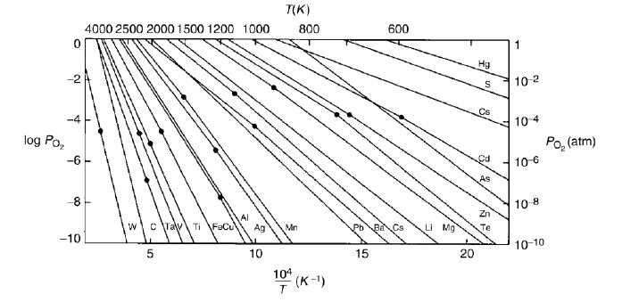 Figure 13.9:
  Figure 14.1: Mixing of three states into
  Figure 14.2:
 Figure 14.5:
  Figure 14.6: Phase Diagram
 Figure 14.7: Properties of an ideal solution
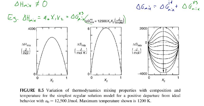 Figure 14.8: Properties of a regular solution
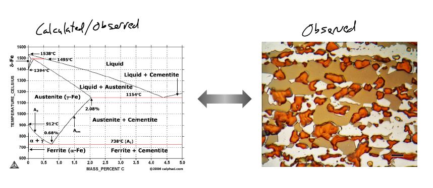 Figure 14.9: Calculated and observed microstructures
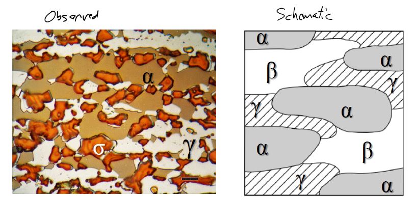 Figure 14.10: Multicomponent heterogeneous (multi-phase) system
 Figure 15.1: Multicomponent heterogeneous and homogeneous systems
 Figure 15.2: Multicomponent heterogeneous (multi-phase) system
 Figure 16.1: Unary (C=1) phase diagram
 Figure 16.3: Binary (c=2) phase diagram
 Figure 16.5: Tie lines on an X-T diagram
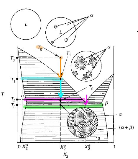 Figure 16.6: Microstructure Evolution
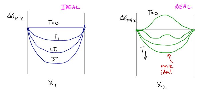 Figure 16.7: Gibbs free energy of mixing for ideal vs real mixtures
 Figure 17.1:
  Figure 17.2:
  Figure 17.4:
 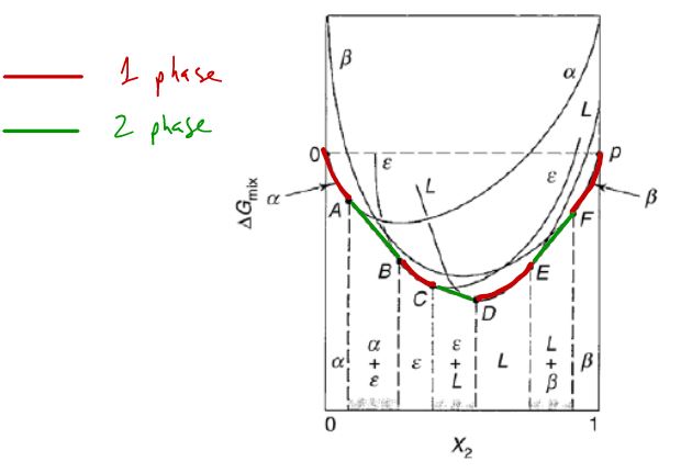 Figure 17.5:
 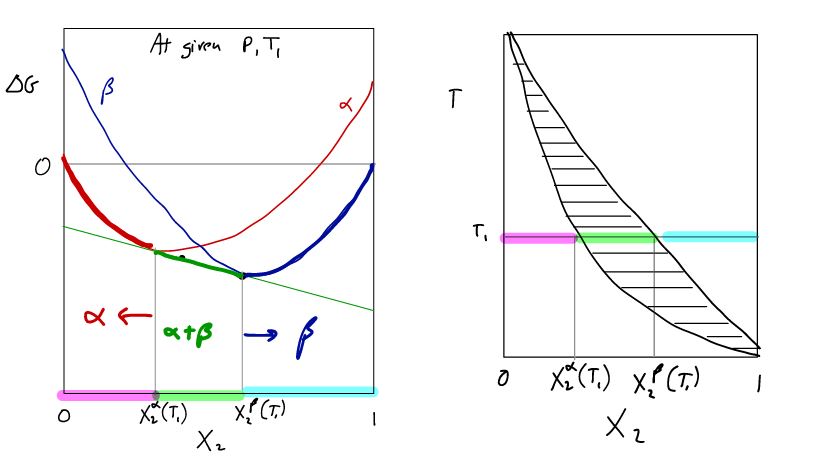 Figure 17.6: Representing single and two phase regions on a phase diagram
 Figure 17.7: G(T) of pure components
 Figure 17.8:
  Figure 17.9:
  Figure 17.10: Variation of mixing properties with composition and temperature for the simplest regular solution model. Maximum temperature is 1200 K, and
  Figure 17.11: Miscibility gap
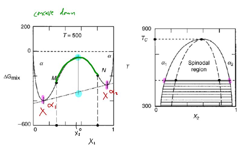 Figure 17.12: Spinodal decomposition


