316-1: Microstructural Dynamics I
Peter W. Voorhees and Kenneth R. ShullDepartment of Materials Science and EngineeringNorthwestern University
1 Catalog Description (316-1,2)
Principles underlying development of microstructures. Defects, diffusion, phase transformations, nucleation and growth, thermal and mechanical treatment of materials. Lectures, laboratory. Prerequisite: 315 or equivalent.
2 Course Outcomes
At the conclusion of 316-1 students will be able to:
- Describe the Kirkendall effect, diffusion in ternary systems, and the importance of short-circuit diffusion.
- Describe the structure of various types of interfaces and the effects these structures have on interfacial energy.
- Apply concepts of mathematics and physics to imperfections, diffusion and phase transformations.
- Use basic concepts of dislocation theory: topology and energetics of dislocations in crystalline materials.
- Exhibit a good understanding of dislocations as related to their type (edge, screw, mixed), stress fields, energies, geometry (bowing, kinks, jogs) and interaction.
- Correlate dislocation motion to plastic flow.
- Describe how the grain size of a material can be controlled by mechanical and thermal processing of materials
- Demonstrate laboratory skills in structural and thermal processing of materials.
3 Diffusion
3.1 Review of the Basic Equations
The diffusion equation describes the evolution of the composition profile with time as the individual components diffuse within a sample. These components can be either atoms or molecules, but for our purposes we'll assume that the diffusing species are atoms (as in a metallic sample). For a binary system of A and B components, we can use either or (the respective concentrations of A and B species in atoms/volume) to describe the composition. These compositions sum to the total atomic concentration, :
If the molar volumes of A and B are equal to one another, then is fixed, so that the following conditions hold:
Note that we are using
as our spatial variable. For a binary A/B alloy we can use either
or
to describe the overall composition of the alloy. The flux of atoms is given by
:
Here
is the
intrinsic diffusion coefficient
for component
and
is the diffusive flux of component
referenced to a given lattice plane in the material. In a binary system there are two intrinsic diffusion coefficients,
and
, and two diffusive fluxes,
and
. The time evolution of the composition is given by the continuity condition that relates a change in local concentration must be related to the spatial derivative of the flux:
The
is obtained by combining Eqs.
3.4 and
3.5:
If the diffusion coefficient is independent of concentration (and hence, independent of as well) then the diffusion equation can be written as follows:
The diffusion equation involves a first derivative with respect to time an a second derivative with respect to distance, so in general we need an initial condition and two boundary conditions. Consider for example the following situation:
- Boundary conditions: for and for
- Initial condition: The concentration jumps discontinuously from to at
With these initial and boundary conditions, the solution to Eq.
3.7 is:
Here is the following diffusion length, which enters into all diffusion problems:
Erf is the
, which is defined formally as follows [
1]:
Note that erf(
) transitions from -1 to large negative values of
to +1 for high positive values of
, as shown in Figure
3.1.
The solution to Eq.
3.8 is shown in Figure
3.2. To show how the concentration profile evolves with time, we have included values of
in the plot.
This program was used to generate Figure
3.2:
figure
figformat % set some defaults so the figures look pretty
z=linspace(-1,1,200);  % These are the z points
w=[0.2,0.4,0.6]; % these are the three values of the normalized diffusion length that we will include in our calculations
c=@(z,w) erf(z/w);  % define a function of two variables, z and w
col={[1,0,0],[0,0.5,0],[0,0,1]};  % these are the three colors (rgb format)
linetype={'-','--','-.'};  % these are the three line types we well used (plain, dashed and dash-dot)
axes
hold on
for i=1:3
    plot(z,c(z,w(i)),'color',col{i},'linestyle',linetype{i})
    legendtext{i}=['$w/L$=' num2str(w(i))];
end
legend(legendtext,'location','best','interpreter','latex')
ylabel('C_{a}')
xlabel('z/L')
ylim([-1.2 1.2])
set(gca,'ytick',[-1,1])
set(gca,'yticklabel',[])  % turn off the y axis tick labls by making 'yticklable' an empty vector
text(-1.15, -1, 'C_{1}','fontsize',16)
text(-1.15, 1, 'C_{2}','fontsize',16)
print(gcf,'../figures/erfsolution.eps','-depsc2') % save as an eps file
We can also consider the situation where we have layer of material at
, which diffuses in the positive and negative directions into the bulk material. In this case the initial and boundary conditions are as follows:
- Boundary conditions: for
- Initial condition: All of the A component is confined to a very layer at , with a surface coverage (atoms/area) of
- Normalization condition: The total amount of material in the sample must be conserved, so if we integrate the concentration profile we must end up with :
In this case the following solution to the diffusion equation is obtained:
Eq.
3.12 is plotted in Figure
3.3 for three different time points.
In many cases all we need to know is the diffusion length,
, in order to understand what is going on at a pretty high level of detail. For example,
describes both the width of interfacial mixing for two materials that are brought into contact with one another (Figure
3.2) and the diffusive broadening of a thin interfacial layer (Figure
3.3). The quantitative interpretation of the diffusion length in these two circumstances is illustrated in Figure
3.4. In Figure
3.4a we plot the interfacial broadening for a thin layer that is diffusing in the positive and negative
directions. The width of the diffusion profile can be characterized by the half-width of the peak,
, evaluated at half the total peak height. In Figure
3.4b we plot the concentration after bars with bulk concentrations of
and
are brought into contact with one another. In this case
is obtained by drawing a tangent to the concentration profile at the midpoint between
and
, and taking
as the horizontal distance between the points where this tangent line reaches concentrations of
and
. The value of
in both cases is quite close to the diffusion length,
.
3.2 Mole Fractions and Volume Fractions
An assumption that we make throughout this text is that the atomic volumes of different chemical species are all identical, equal to In reality, this is almost never exactly true. Fortunately, it doesn't really matter when thinking about diffusion because we can always work with volume fractions instead of mole fractions. In a generalized formulation the molecular volumes of the A and B molecules are given by multiplying the reference volume by a factor of , which is not necessarily the same for each molecule:
We can relate concentrations to mole fractions and volume fractions by considering a binary A/B system with total atoms. Of these, are A atoms and are B atoms. Multiplying by the the atomic volume gives the total volume of each component. The total volume of A atoms is and the total volume of B atoms is . From these expressions we obtain the following for , the volume fraction of A atoms in the system:
where is the total volume of the system. Note that we have used and . Throughout the rest of this text we generally assume that In the case where and/or are not equal to one we can define renormalized concentrations, and that describe the concentration of subunits of volume These fluxes are related to the atomic fluxes, and by multiplying by the appropriate value of :
The renormalized fluxes, and are obtained by a similar normalization:
Fick's first law still holds for these renormalized fluxes and concentrations, since we are just multiplying each side of Eq.
3.4 by
. Fick's second law applies for a similar reason. We can also use Eq.
3.15 to substitute
for
:
The bottom line of all this is that Fick's second law still applies, with same diffusion coefficient used for the case where the atomic volumes are equal, provided that we simply replace concentrations with volume fractions.
3.3 Vacancy Diffusion Mechanism
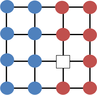
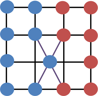
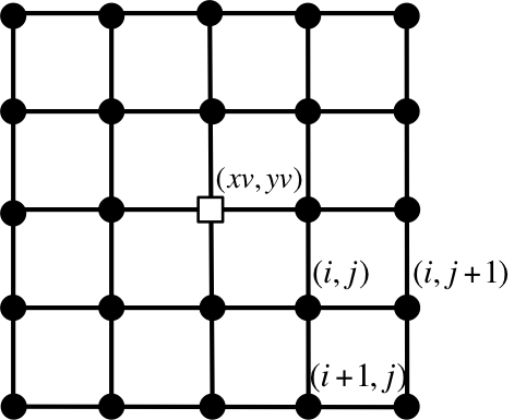
Figure
3.5 shows the output of a vacancy diffusion simulation of the interdiffusion between two materials. Vacancies move when an atom from an adjacent site moves into the vacancy. The resulting net motion of the atoms provides a means for diffusive mixing across an interface, and this is the process being illustrated in Figure
3.5 If the probability of hopping into a vacancy is different for A and B atoms, then
, and we need to consider additional effects. These are described below in our discussion of the Kirkendall effect.
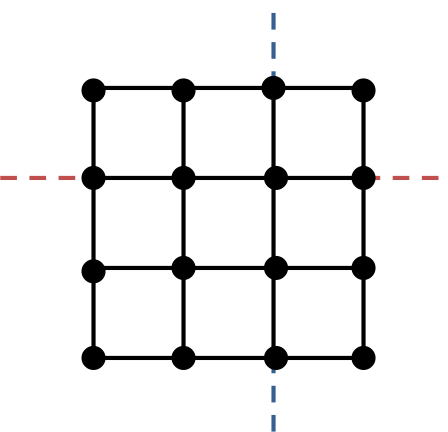
The following program was used to generate the images shown in Figure
3.5.
tic % start a time so that we can see how long the program takes to run
n=30;  % set the number of boxes across the square grid
vfrac=0.01;  % vacancy fraction
matrix=ones(n);
map=[1,1,1;1,0,0;0,0,1];  % define 3 colors:  white, red, blue
figure
colormap(map)  % set the mapping of values in 'matrix' to a specific color
caxis([0 2]) % range of values in matrix goes from 0 (vacancy) to 2
% the previous three commands set things up so a 0 will be white, a 1 will
% be red and a 2 sill be blue
matrix(:,n/2+1:n)=2;  % set the right half of the matrix to 'blue'
i=round(n/2);   % put one vacancy in the middle
j=round(n/2);
matrix(i,j)=0;
imagesc(matrix); % this is the command that takes the matrix and turns it into a plot
t=0;
times=[1e4,2e4,5e4,1e5];
showallimages=1; % set to zero if you want to speed things up by not showing images,  set to 1 if you want to show all the images during the simulation

%% now we start to move things around
vacancydiff.matrices={};  % makea blank cell array
while t<max(times)
    t=t+1;
    dir=randi([1 4], 1, 1);
    if dir==1
        in=i+1;
        jn=j;
        if in==n+1; in=1; end
    elseif dir==2
        in=i-1;
        jn=j;
        if in==0; in=n; end
    elseif dir==3
        in=i;
        jn=j+1;
        if jn>n; jn=n; end
    elseif dir==4
        in=i;
        jn=j-1;
        if jn==0; jn=1; end
    end
    % now we need to make switch
    neighborix=sub2ind([n n],in,jn);
    vacix=sub2ind([n n],i,j);
    matrix([vacix neighborix])=matrix([neighborix vacix]);
    if showallimages
        imagesc(matrix);
        drawnow
    end
    if ismember(t,times)
        vacancydiff.matrices=[vacancydiff.matrices {matrix}]; % append matrix to output file
        imagesc(matrix);
        set(gcf,'paperposition',[0 0 5 5])
        set(gcf,'papersize',[5 5])
        print(gcf,['vacdiff' num2str(t) '.eps'],'-depsc2')
    end
    i=in;
    j=jn;
end
vacancydiff.times=times;
vacancydiff.n=n;
save('vacancydiff.mat','vacancydiff') % writes the vacancydiff structure to a .mat file that we can read in later
toc
3.4 Kirkendall Effect
The geometry of the Kirkendall experiment (1947) is shown in Figure
3.6 [
7]. In the experiment a small block of brass (70% copper, 30% Zn) was surrounded by inert, Molybdenum (Mo) wires. The sample was then coated with copper, and heated to a high temperature to allow atoms within the material to diffuse. In the measurement, the distance,
, between the Mo markers decreased as a function of time. This result implies that the flux of Zn out of the brass portion of the sample is larger than the copper flux back into the brass from the outside.
Diffusion does not need to occur by a vacancy motion in order for the Kirkendall effect to be observed, all that is needed is an asymmetry in the diffusion coefficients of the individual components in the material. However, for our purposes we will assume for now that diffusion occurs by a vacancy hopping mechanism. This assumption is valid for the original Kirkendall experiment, and it also enables us to make a connection to the relevant microscopic diffusion mechanisms. It is an excellent example of the structure/property relationships that define the field of materials science.
Our starting point is to assume that the vacancy concentration remains at equilibrium, so that the total number of lattice sites (including vacant sites) remains constant. A consequence of this assumption is that the fluxes of of A atoms, B atoms and vacancies must sum to zero:
Rearrangement of this equation, in combination with Fick's first law (Eq.
3.4) and the requirement that
leads to the following:
The situation for
is illustrated in Figure
3.7. In this case the net vacancy flux is negative (to the left), and has a maximum magnitude at the point where the concentration gradient is the largest. Because the vacancy flux varies with position, there will be a time dependent increase or decrease in the local vacancy concentration that can be obtained from a site conservation equation similar to Eq.
3.5:
This results in a net depletion of vacancies in some regions of the sample (the right in Figure
3.7c) and a net supersaturation of the vacancy concentration in other regions of the sample (the left in Figure
3.7c). In most cases processes exist that enable these concentration variations to be eliminated, by the creation of vacancies at the right portion of the sample and the destruction of vacancies at the left portion of the sample. Typically, these processes involve the addition or removal of vacancies to the core of a dislocation.
3.5 The Interdiffusion Coefficient
In general, a material flux, , within a material can be related to a velocity, . This velocity is obtained simply by multiplying by the reference volume, , that is used to define the diffusive flux: ():
The relevant velocity for us is a net, material velocity with respect to a set of inert markers, corresponding, for example to markers shown in the schematic representation of the Kirkendall experiment (Figure
3.6). It is easy to see from this picture, that if there is a net material flux to the right (in the positive direction), the result will be a net motion of the markers to the left. The value of
, the net velocity of the markers with respect to the ends of the samples, is determined by using -
as the relevant flux in Eq.
3.21:
We will often find it useful to use mole fractions instead of concentrations in our expressions, so we need to keep the following relationship in mind:
with
=A we can differentiate Eq.
3.23 to obtain:
We can now combine Fick's first law (Eq.
3.4) with Eqs.
3.22 and
3.23 to obtain:
This is the velocity that individual planes are moving with respect to a fixed position in the sample that is far from the interface (the ends of the sample, for example). The fluxes obtained from Fick's first law are defined in terms of a reference plane that is moving with a velocity . We can also define fluxes of A and B atoms across stationary planes, and we refer to these fluxes as and . We can get by adding to , where is the net flux of A atoms across a fixed plane in space due to the lattice plane velocity:
We can combine this expression with Eq. for to get:
With
, we can combine Eqs.
3.24 and
3.27 to obtain:
After a bit of algebra, keeping in mind that , we obtain the following:
Now we can define an
interdiffusion coefficient
,
:
with this definition we have:
A similar approach can be used to show that
and that the same value of
can be used to relate
to
. In addition, this same value of
now appears in Fick's second law, where we can see from Eq.
3.30 that the value of
is generally going to be composition dependent. The concentration profile therefore evolves according to the time-dependent solution of the following form of Fick's second law:
3.6 Connection to thermodynamics
At equilibrium the chemical potential of component
,
is a constant. If
is not constant, then we must have diffusive fluxes as the system move towards equilibrium. It's not a gradient in concentration that generates the flux, it's really the gradient in the chemical potential,
. A simple example illustrating this point is the abrupt change in concentration that exists at an equilibrated interface between two coexisting phases, shown as the
and
phases in Figure
3.8. Even though there is a large composition gradient at the interface, there is no diffusion for an equilibrated system because the chemical potential is spatially uniform.
This example illustrates the fact that diffusion involves more than just concentration gradients, but involves thermodynamic factors as well. In order to account for these we need to revisit Fick's first law, but write things in terms of the chemical potentials. The flux of B atoms is can be written as the product of
and a diffusive velocity
where
is the average velocity at which the B atoms are moving. This velocity is related to the concentration gradient by a
,
:
Note that must be positive. Atoms always move down a chemical potential potential gradient, although in some cases diffusion may take place up a concentration gradient (more on this in 316-2). We can use the previous expression for to obtain the following expression for the diffusive flux of B atoms:
We can use Eq.
3.24 to write this in terms of a concentration gradient:
Comparing to Fick's first law (Eq.
3.4), we obtain the following for
:
We see the this intrinsic diffusion coefficients involves purely kinetic parameter (the mobility, ), and a thermodynamic parameter (the derivative of with concentration). As discussed in more detail in 315 (see the sectional on Type II (binary) phase diagrams), chemical potentials are most commonly expressed in terms of activity coefficients in the following way:
Here is the standard state, which is generally defined to be zero for a pure material at thermodynamic equilibrium. This equation can be used to write the chemical potential derivative in the following way:
3.7 Tracer Diffusion Coefficients
The tracer diffusion coefficient can be viewed as the diffusion coefficient for a dilute species. The matrix in which the tracer is diffusing can itself be a mixture of different elements, as we illustrated schematically in Figure
3.9. The following features of the tracer diffusion coefficients are important to keep in mind:
- Like mobilities, tracer diffusion coefficients are purely kinetic parameters.
- Tracer diffusion coefficients will depend on the local composition (the relative amount of A and B atoms in a binary alloy, for example).
- A binary A-B alloy there are two, independent, composition-dependent tracer diffusion coefficients. If the tracer species is chemically identical to atom A, then we refer to the tracer diffusion coefficient as . If the tracer species is chemically identical to atom B, then we refer to the tracer diffusion coefficient as .
By definition, tracer diffusion coefficients are are defined in the dilute limit, where the activity increases linearly with concentration in a way that is given by the Henry's law coefficient, . We'll illustrate things by assuming that the tracer is chemically identical to B. In this case we express Henry's law in the following way:
From Eq.
3.38 we obtain the following expression for the chemical potential derivative in the dilute (Henry's law) regime.
The tracer diffusion coefficient for the B atoms is related to the mobility by the following expression:
The general relationship between
and
, valid for all compositions, and not just in the Henry's law regime, is obtained by comparing Eqs.
3.36 and
3.41:
As a result, whenever is proportional to . This is the case when is very small (Henry's law regime), and when is close to 1 (Rault's law regime), but it is not necessarily true or intermediate values of .
3.8 Summary of Diffusion in a Binary System
We have defined three interrelated types diffusion coefficients: , and . Here we provide a brief summary of these different diffusion coefficients and the relationships between them.
- : The interdiffusion coefficient (often referred to as the mutual diffusion coefficient). If you are interested in the time-dependent evolution of the composition profile, this is the diffusion coefficient that you use when you are solving the diffusion equation:
note that for a binary system, we only need to specify one of the compositions, since . Also note that in general, depends on the composition, so cannot be treated as a constant.
- and : The intrinsic diffusion coefficients for the individual components. These are important for two reasons. First, they are needed if you want to describe motions of atomic planes relative to the external boundaries of the sample (the Kirkendall effect). This motion was determined from the the atomic fluxes relative to atomic planes, as opposed to fixed points in space. These fluxes are determined by the appropriate intrinsic diffusion coefficient. For example, for the B component, we have:
Also, predictive models of interdiffusion are generally based on the relationship between these intrinsic diffusion coefficients and the interdiffusion coefficient through the following expression:
- and : The tracer diffusion coefficients for the individual components. Imagine a single atom in a homogeneous material. The tracer diffusion coefficient describes the probability that the atom has diffused a certain distance in a given period of time. These diffusion coefficients are purely kinetic parameters, and can be expressed in terms of a mobilty:
Unlike the interdiffusion and intrinsic diffusion coefficients, they are not affected by the thermodynamics of the system. In general, values of the tracer diffusion coefficients will depend on the concentration of the material in which the tracer atoms are diffusing. The special cases of at and at are self diffusion coefficients. The intrinsic diffusion coefficients are related to the tracer diffusion coefficients through the following relationship:
3.9 Diffusion in Ternary Systems
Atomic diffusion in ternary systems is driven by chemical potential gradients, just as it is does in binary systems. In systems with more than two components, however, the composition is no longer specified by a single composition variable. Some interesting effects can be observed in this case, as exemplified by carbon diffusion in Fe-Si-C ternary alloys . The carbon chemical potential is now a function of the concentration of both the silicon and carbon in the alloy:
The diffusion coefficient of carbon is much larger than the diffusion coefficient for silicon (
), so we can assume that the silicon remains stationary during a diffusion experiment, as shown in Figure
3.10. Silicon and carbon have a unfavorable thermodynamic interaction within the alloy, so
increases with increasing silicon content,
. In order for the carbon chemical potential to remain constant across and interface between two regions of differing Si content, the carbon concentration in the region with low Si content needs to be smaller than the carbon concentration in the region with high Si content. This chemical potential discontinuity at the interface is eliminated by the jump of carbon atoms from the left (high Si side) to the right (low Si side) of the interface. Diffusion then continues from left to right, down the carbon potential gradient that has been established.
3.10 Crystal Defects and High Diffusivity Paths
“Crystals are like people. It is the defects in them which tend to make them interesting.” - Colin Humphreys
Real crystals are never perfect, and they always contain some sort of defects. These defects can be classified into four categories, based on their dimension:
- 0-dimensional (point) defects: These include missing atoms (vacancies), or atoms in location where they would not be in a perfect crystal structure (interstitials or substitutional impurities. From purely thermodynamic considerations we know that point defects must exist at some finite concentration for temperatures above 0K.
- 1-dimensional (line) defects: These are dislocations.
- 2-dimensional (planar) defects: These include grain boundaries, which are internal interfaces between regions of different crystalline orientation, and the external surfaces of a material.
- 3-dimensional (volume) defects: These are geometric imperfections in a material, like pores and cracks. We don't consider these types of defects in this class, but they become very important when we discuss the fracture properties of bulk, brittle materials in subsequent courses.
As illustrated in Figure
3.11, dislocation, grain boundaries and surfaces are associated with a more open structure. As a result diffusion along these defects is much faster than in the bulk of the material.
4 Dislocations
Plastic deformation of a crystalline solid occurs by the motion of dislocations, which are one dimensional defects in the crystal structure. In general, deformation of a material occurs by shear along specified planes called slip planes. An illustration of this effect in single crystal aluminum is shown in Figure
4.1. The material in this image is being deformed in tension, but the slip occurs along suitably oriented planes that are experiencing a high degree of shear.
When a stress is applied to a single crystal, deformation takes place when the
,
, on an appropriately aligned shear plane exceeds a critical value, referred to as the
critical resolved shear stress
,
. The relationship between the tensile stress,
and the resolved shear stress is illustrated in Figure
4.2. In mathematical terms we have:
where is the angle between the tensile axis and the slip plane normal, , and is the angle between the tensile axis and the slip direction, .
Values of this quantity for different single crystals are shown in Table
1. For the materials with close packed crystals structures on this list (fcc and hcp), the value of
is about four orders of magnitude less than the shear modulus,
.
.
Table 1: Critical resolved shear stress for single crystals (Read-Hill, “Physics of Metals Principles”, chap. 4 (1964).
|
Metal
|
Structure
|
(psi)
|
(Pa)
|
(psi)
|
(Pa)
|
|
Al
|
fcc
|
3.9x10
|
27x10
|
148
|
1.0x10
|
|
Cu
|
fcc
|
7.0x10
|
48x10
|
92
|
0.64x10
|
|
Mg
|
hcp
|
2.4x10
|
17x10
|
63
|
0.44x10
|
|
Zn
|
hcp
|
5.6x10
|
38x10
|
26
|
0.18x10
|
|
-Fe
|
bcc
|
9x10
|
27x10
|
4000
|
28x10
|
Why is the force to deform a single crystal so low? We'll start by considering what we would expect for the critical resolved shear stress if the shear deformation were to occur by the sliding of atomic planes over one another, as shown conceptually in Figure
4.3. We refer to the stress required to slide these planes over one another as the dislocation-free critical resolved shear stress,
We'll start by reminding ourselves of the definition of a shear strain, illustrated in Figure
4.4. In shear deformation, two parallel surfaces separated by a distance,
, are translated by an amount
with respect to one another. If the deformation occurs in the x-y plane, we refer to the shear strain as
, which is given by:
For a linearly elastic material, the shear stress, is proportional to , with the shear modulus defined as the ratio of shear stress over shear strain:
In Figure
4.5 show a schematic representation of the stress as a function of displacement for the atomic planes shown in Figure
4.3. The stress function has the following features:
- The stress is a periodic function, with the stress repeating every time the displacement is increased by an amount equal to , the distance between atoms along the slip direction.
- The stress is equal to zero at the stable equilibrium positions at , etc.
- For the stress is positive because we need to apply a stress to move the atoms out of their stable equilibrium positions.
- At the system is at an unstable equilibrium. The stress is also equal to zero at this position, but the equilibrium is unstable because any slight perturbation in the displacement will cause the atomic plane to fall back into an equilibrium position at or .
- The maximum stress is at . The stress actually reverses sign for , since a stress must be applied to avoid having the atoms fall into the equilibrium position at .
The simplest mathematical expression for the shear stress that has the right periodicity is a sinusoidal function:
Now we need to figure out what the constant
is in terms of actual material properties. For small displacements the material is in the linear regime, and we can use the definition of the shear modulus (Eq.
4.3) to obtain the following:
Comparison of Eqs.
4.4 and
4.5 gives
, so the shear stress becomes:
The critical resolved shear stress in this picture corresponds to the maximum value of
, equal to
. The interplanar spacing,
is comparable to
. (We're not going to worry about the exact numerical factor here, since we're just aiming to get an approximate expression for
). We take
and
to end up with the following expression for the ideal critical resolved shear stress,
, which is the value of the critical resolved shear stress we would expect to have if dis:
In reality,
, so this picture of atomic planes sliding over one another can't be correct. What is really going on here? The answer is that slip occurs by the motion of dislocations, not by the concerted motion of entire planes of atoms across one another. The concept of slip by dislocation motion can be illustrated conceptually by the force required to slide a carpet across a floor. If the friction between the rug and the floor is very high, it's going to be very difficult to move the rug along the floor simply by grabbing it from one end and pulling. This situation is analogous to sliding atomic planes across one another as illustrated in Figure
4.3. If the rug just needs to be moved a small distance it is much easier to create a wrinkle at one end of the rug and move it to the other end of the carpet. At the end of the process, the carpet has moved by a length equal to the length of extra carpet stored in the wrinkle. Dislocations are line defects in crystalline materials that are analogous to these wrinkles.
4.1 Edge Dislocations
The easiest type of dislocation to visualize is an edge dislocation.
A dislocation is formed by slipping part of the top half of a crystal relative to the bottom half by the application of a shear stress,
, as illustrated schematically in Figure
4.7. The
corresponds to the interface between the slipped and unslipped regions of the sample. An edge dislocation can be viewed as the termination of an extra half plane of atoms, and is illustrated for a simple cubic lattice in Figure
4.8.
Motion of an edge dislocation is illustrated in response to an applied shear stress is illustrated in Figure
4.9. Note that for every atom moving away from its equilibrium on one side of the dislocation core, there is an equivalent atom moving toward an equilibrium position on the other side of the dislocation core. In energetic terms, for every atom that must be forced out of its lowest energy position, there is atom moving toward its lowest energy position. As a result the energy changes cancel (or very nearly so), and the energy barrier to moving a dislocation is much less than the barrier to slide surfaces across one another. As a result the net force to move a dislocation is very small. The stress needed to move a dislocation is generally much less than
, and is as low or lower than the observed critical resolved shear stress for single crystals.
The relative displacement of the two halves of the crystal caused by the motion of a single dislocation through it is the
,
, which is the single most important characteristic of the dislocation. For an edge dislocation
is perpendicular to the dislocation line, which we represent by the unit vector
(the
)
. Note that dislocations of opposite sign moving in opposite directions give the same final shear. This is illustrated by comparing Figures
4.9 and
4.10, which both result in the final deformed state of the material. Finally, when two edge dislocations with opposite Burgers vectors (
and
) meet on the same glide plane, they annihilate each other (see Figure
4.11).
4.2 Screw Dislocations
As with edge dislocations, a screw dislocation line marks the boundary between 'slipped' and 'unslipped' regions of the sample, but for a screw dislocation the displacement described by
is parallel to the dislocation line,
. (Note that in order to simplify our notation, we'll refer to
, the magnitude of the Burgers vector, simply as
in this text. A schematic representation of a the displacements associated with a screw dislocation is shown in Figure
4.12.
Figure
4.13 illustrates the the motion of a screw dislocation through a crystal. In this case the dislocation moves from the front of the crystal to the back of the crystal. The net effect of this motion is for the top and bottom halves of the crystal to be displaced to the right, by an amount and in the direction given by the Burgers vector. This figure illustrates the following:
- When a dislocation line travels through a material, the motion of the line traces out a plane.
- The relative displacement between the material on either side of this plane is given by the Burgers vector .
Note that this is true for ANY dislocation (edge, screw, or mixed).
4.3 The Burgers Circuit
In the previous section we have described some of the basic features of edge and dislocations, and have shown that they differ in the relationship between the orientation of the Burgers vector with respect to the dislocation line. Now we introduce a formal procedure that can be used to determine the value of
for any dislocation. The procedure is based on the use of a
, as described here:
- Draw a circuit around the dislocation line that starts end ends at the same point. A 'right handed' convention is typically used to describe the direction that we take the circuit. (Clockwise looking along the direction of , counterclockwise if is pointed at you).
- Repeat the procedure, using the same numbers of atomic steps in each direction in a perfect crystal.
- The Burgers vector is the vector connecting the start and end positions for the circuit drawn in the perfect crystal.
Use of the procedure is illustrated in Figure
4.14 for an edge dislocation with an extra half plane in the top half of the crystal. The circuit around the dislocation begins and ends at point a and proceeds as follows:
- Move four steps down (a to b)
- Move three steps to the right (b to c)
- Move four steps up (c to d)
- Move four steps to the left (d back to a)
When this same procedure is repeated in the perfect crystal we end up at point e, which is one step to the left of our starting point at point a. Our convention is to define the
as the vector starting at point a and ending at point b. When the procedure is repeated for a dislocation where the half plane is in the bottom half of the crystal we end up with the Burgers vector pointing in the opposite direction, as shown in Figure
4.15.
In Figure
4.16 we repeat the same process for a screw dislocation. In this example we have defined the direction of
so that the dislocation is pointed toward the bottom of the figure. The procedure for determining
is as follows:
- Draw a circuit in the clockwise direction (viewed from the top, so we are looking in the direction of ) around the dislocation line. The circuit begins and ends at point a.
- Repeat the circuit in a perfect part of the crystal. The circuit begins at point and ends at point .
- The Burgers vector is obtained as the vector that starts at and ends at
Note that
is parallel to
, as it must be for a screw dislocation, but that
and
are pointed in opposite directions,
i.e., they are anti-parallel. With our convention of drawing the
from the starting point to the ending point of the Burgers circuit in the perfect crystal, right handed screw dislocations have negative Burgers vectors and left handed screw dislocations have positive Burgers vectors. The left handed version of the dislocation shown in Figure
4.16 is shown in Figure
4.17.
4.4 The cross product
The concept of the Burgers circuit is a useful formalism that can always be used to specify the Burgers vector for a given dislocation. The confusing part about the procedure is that the sign of the Burgers vector depends on some arbitrary conventions that are not used the same way by everyone. For example, our convention is to define
as the vector linking the start to the finish of the Burgers circuit in the perfect crystal (linking points s to f in Figure
4.16), but you can find plenty of other people who draw the vector the other way around (drawing
from point f to point s). Nevertheless, we remove any ambiguity by always using this 'start-to-finish' definition for the Burgers vector. Similarly, we remove ambiguity regarding the direction in which we take the Burgers circuit by always doing it the same way. In our case we use the right hand rule, directing our thumb along
and drawing the circuit in the direction in which our fingers are pointing.
Unfortunately, the ambiguity introduced by our definition of the direction of
along the dislocation line is impossible to remove. In figure
4.16 we defined
so that it points along the negative z direction, but there's no reason that we couldn't have defined
so that it is directed in the positive z direction instead. We end up with a Burgers vector that points in one of two opposite directions, depending on how we define
in the first place. The good news is that
, the vector cross product of
and
is independent of our convention for defining the direction of
. As a reminder, the vector cross product between vectors
and
is defined as follows, as illustrated in Figure
4.18:[
#_cross_2014]
Here is a unit vector in the direction perpendicular to the plane containing and . It's orientation is defined using the right hand rule: We place our right hand along , with our fingers oriented in the positive direction. Our right thumb is then pointed along .
When defined in this way, has the following properties:
- Because redefining to have the opposite orientation also changes the orientation of , the negative signs cancel and we end up with a value for that is independent of the way that we choose to define .
- For a pure screw dislocation, or . In either case, = 0.
- For an edge dislocation, the magnitude of is equal to the , the magnitude of Burgers vector. In addition, points toward the extra half plane.
This last point is perhaps the most important one, because it provides an easy way to figure out how the extra half plane is oriented in an edge dislocation, once we specify the orientations of
and
. We just use the right hand rule, cross
into
, and our thumb will be pointed along the direction of the extra half plane. To convince yourself that this actually works, you can try it with the edge dislocations pictured in Figures
4.14 and
4.15.
With our convention for using the Burgers circuit to obtain (Right-hand-rule, start to finish), we have the following relationships between and :
- Right-handed screw dislocation: and point in opposite directions.
- Left-handed screw dislocation: and point in the same direction.
- Edge dislocation: perpendicular to , points to the extra half plane.
4.5 Connection to the Crystal Structure
The Burgers vector must correspond to an atomic repeat distance in the crystal structure. As we show below, the energy of a dislocation is proportional to the square of the magnitude of the Burgers vector. For this reason the Burgers vector will correspond to closest atomic distance in crystal structure. As shown in Figure
4.19, the Burgers vector is half the unit cell diagonal for the BCC structure, and half the face diagonal of the unit cell in the FCC structure.
4.6 Dislocation loops
A dislocation cannot terminate within a crystal, although it can terminate at a grain boundary or crystal surface. Also, while the Burgers vector along a given dislocation is constant, the dislocation itself is not necessarily a straight line. In other words,
is fixed, but
can change as the direction of the dislocation changes. Consider for example the dislocation loop shown in Figure
4.20.
Exercise: What happens to the shape of the crystal in Figure
4.20 if the loop contracts to nothing and disappears?
Solution: The dislocation just disappears, and a perfect crystal (at least in this region) is recovered.
4.7 Dislocation Density
The following two definitions of the
are often used:
- Total line length of dislocations per volume.
- The number of intersections that the dislocations make with a plane of unit area.
Both definitions give dislocation densities with units of 1/area, and are equivalent if the dislocations are straight. Typical dislocation densities are as follows:
- A well annealed metal: /cm.
- Plastically deformed metal: can be as high as /cm.
- Ceramics: Much lower, typically 10/cm.
- Si used in microelectronics: dislocation density of zero! Macroscopic single crystals are typically grown without a single dislocation. The down side of this is that Si is very brittle, since there is no plastic deformation mechanism.
4.8 Dislocation Motion
4.8.1 Dislocation Glide
Dislocation
(which is sometimes referred to simply as slip) corresponds to dislocation motion within a
that contains along the plane that contains both the Burgers vector,
and the sense,
, of the dislocation. For an edge dislocation or a dislocation with mixed edge and screw character, a single slip plane exists that is perpendicular to the vector
, given by the cross product of
and
(see Figure
4.18). Slip does not require atomic diffusion, and so is not strongly temperature dependent. For an edge dislocation it occurs when the extra half plane of atoms reattaches to a new atomic plane, moving the half plane by a distance equal to
. The process is illustrated schematically in Figure
4.21.
For a pure screw dislocation, because
and
are collinear, a variety of glide planes are available. As a result, screw dislocations can more easily navigate their way around obstacles (like a precipitate particle) by changing the slip plane on which they are moving. The process is called
and is illustrated schematically in Figure
4.22. This illustration could correspond, for example, to the motion of a screw dislocation with
oriented along the
direction that moves along the
plane initially, switches to the
plane and then begins moving again in the
plane. (Note - if you forget the Miller index notation for planes and directions, the Wikipedia page [
#_miller_2014] is a useful refresher).
4.8.2 Dislocation Climb
Edge dislocations can climb
out of the glide plane by the addition or subtraction of vacancies to the dislocation core. The process is illustrated in Figure
4.23 for a situation where
is directed toward the top of the figure (
i.e. the extra half plane is above the glide plane). In this example an atom at the end of the extra half plane jumps into a vacancy. The net result is that the vacancy is destroyed, and the dislocation climbs up, away from the initial glide plane. Because the process requires the diffusive hopping of atoms from one site to another, climb is a thermally activated process that becomes more important at elevated temperatures.
If dislocations climb in the direction of
(in the direction of the extra half plane) as illustrated in Figure
4.23, vacancies are destroyed. If they climb in the other direction (adding atoms to the extra half plane instead of removing them), the opposite occurs and vacancies are created. Dislocation climb therefore provides an mechanisms for equilibrating the vacancy concentration. For metals it is the process that allows us to assume that the vacancy concentration remains at equilibrium, and important assumption of our analysis of the Kirkendall experiment in Section
3.4.
4.9 Dislocation Energy
Dislocation disrupts the regularity of the lattice, and introduces strain into the sample. The strain field that results from the presence of a dislocation has a very long range, and can easily be more than 100 times the unit cell dimension. As a result the total strain energy is very large as well. This strain field and the energy associated with it is important because it provides a mechanism for dislocations to interact with one another over long distances. In essence, dislocations 'talk' to each other through these strain fields.
4.9.1 Screw Dislocations
For a screw dislocation we can use some simple concepts to calculate this strain energy, so we'll start with this example. Our starting point is that the material surrounding a screw dislocation is in a state of pure shear, with shear deformation as defined in Figure
4.4. We see this by considering a cylindrical portion of the material around a screw dislocation, using the illustration in Figure
4.24. The displacement applied across the dislocation is given by the Burgers vector,
(Figure
4.24a). (When referring to the magnitude of the Burgers vector we'll drop the vector symbol and just use the
). If we unwrap the circumference of the cylinder at a distance
from the dislocation line (Figure
4.24b) we see that the shear displacement of
is applied over a distance of
. The cylinder has been unwrapped in the circumferential direction,
i.e. the
direction, and the displacement is along the
direction so we have the following for th shear strain,
:
The distortion is pure shear, with a shear strain at a radius of given by the following:
Note that as . The strain can't really go to infinity, so we have a problem here that we're going to have to deal with eventually. The elastic stress is obtained by multiplying by the shear modulus:
The elastic strain energy per unit volume, is obtained from the following expression:
Dimensionally this makes sense, since has units of force/area, or energy/volume.
We can combine Eqs.
4.9 and
4.11 to obtain the following:
Because the strain energy is radially symmetric, we can get the energy per unit length of the dislocation () by integrating all values of . Because the area element in radial coordinates is , we have:
Substituting
from Eq.
4.12 into this equation gives:
After integration we obtain:
We have a problem here because . This is because for , the shear strain goes to infinity and we can no longer use the simple, continuum picture of linear elasticity to describe what is going on. Instead what we typically do is separate out a core energy, that corresponds to the strain energy inside some small core radius, . We do this simply be adding to and replacing the lower bound on the integration from 0 to .
We can generally choose so that it is large enough so that our assumption of linear elasticity holds for , yet it is small enough so that is a relatively small fraction of the overall dislocation energy. In this case we can ignore the core energy and approximate the dislocation energy as follows:
4.9.2 Edge Dislocations
The stress field for an this case is much more complicated, as illustrated in Figure
4.25. The distinctive features of the strain field are as follows:
- In the slip plane itself the material is in a state of pure shear.
- Above the slip plane there is compressive component to the strain field.
- Below the slip plane there is a tensile component to the strain field.
A more detailed calculation shows that the strain still decays as , with an expression for the edge dislocation energy per length that is similar to the expression obtained for a screw dislocation:
Here, is Poisson's ratio. Typically for most metals.
The conceptual picture shown in Figure
4.25 is useful, but we can do a little bit better by reminding ourselves of some definitions pertaining to a stress state. A two-dimensional stress state in the x-y plane has three independent components of the stress: the shear stress,
, and two normal stresses,
and
, as shown in Figure
4.26. In Figure
4.27a the regions around an edge dislocation where stress components have different signs are illustrated. Figure
4.27b has similar information, but in this case we plot contours of equal stress for each of the three stress components,
,
and
.
4.9.3 General Comments
The following general comments are valid for edge, screw and mixed dislocations:
- Elastic strain energy scales with so it has a very long range.
- The boundary conditions matter, so the energy depends on the shape of the sample. A small crystal with low value of will have a lower dislocation energy than a large crystal with a very large value of .
- Energy scales as . Dislocations with small values of are therefore preferred, which is why the Burgers vector in a material corresponds to the smallest interatomic spacing in the material.
- Energy scales as . Energy is proportional to the length of the dislocation. This means the strain energy will decreases as the line length decreases.
This last point seems trivial at first, but it has some important consequences. Consider for example a dislocation loop. If the radius of a circular loop decreases, the energy associated with the loop will decrease as well. There's a line tension acting on the loop causing it to contract. This tension is like the tension in a rubber band that once to squeeze things inward, and can be viewed as a driving force for the dislocation loop to shrink in size. An applied stress can cause a dislocation loop to grow instead of shrink, and this will be considered later.
Let's compare some numbers to see how the dislocation energy compares to the energy of other defects, like vacancies, for example. To do this we'll estimate the energy per atomic length along a screw dislocation line by taking
in Eq.
4.17. We'll also assume typical values for the other parameters in the expression for
, with
=0.3 nm,
nm.
, and
Pa:
A more convenient energy scale on an atomic basis is the electron volt, which we obtain from the energy in Joules by dividing by the electron charge (1.6x10 C). In these units the energy per atom along the dislocation line is 2.8 eV. This energy of comparable magnitude to typical vacancy formation energies of 1eV, but is actually larger because of the nature of the long-range strain field that is produced around a dislocation.
4.10 Dislocation Line Tension
An energy per unit length has dimensions of a force. The dislocation energy per unit length is therefore equivalent to a force, or tension, exerted by the dislocation. We refer to this line tension as :
This line tension is a one dimensional analog of the interfacial free energy, with units of energy per length instead of energy per area. The comparison is summarized in Table
2.
Table 2: Comparison of line tension and the interfacial free energy.
|
Quantity
|
Energy units
|
Force Units
|
|
|
J/m
|
N
|
|
|
J/m
|
N/m
|
The line tension itself is a force, and it gives rise to a force per unit length acting perpendicular to a curved dislocation line, in the same way that the interfacial free energy results in a pressure difference (force per unit area) across a curved surface. The work done against this one dimensional pressure, which we refer to as
is equal to the increase in free energy associated with the increased length of the dislocation line. By considering the graphical construction shown in Figure
4.28:
Rearrangement gives the following expression for :
4.11 Effect of Applied Stress
The line tension acts to decrease the area of a dislocation loop, but we need loops to expand in order for a material to plastically deform. So how does an applied stress induce a force on a dislocation? The relevant shear stress is the component of the shear stress in the glide plane that operates in the direction of
. This shear stress is the resolved shear stress,
. This applied shear stress results in an additional force per unit length,
. It's easiest to visualize the relationship between
and
for an edge dislocation, as we illustrate in Figure
4.30. To do this we use an energy balance. When the dislocation has propagated across the entire sample a total applied shear force,
, results in a net translation of the material above the slip plane by an amount given by the Burgers vector,
. The total work put into the system is simply
(force times displacement). With
this total work is:
This work goes into moving the dislocation, and must be equal to the force applied to the dislocation multiplied by the distance the dislocation moves as it translates across the sample. In our notation this distance is the sample width, , so we have:
Equating these two expressions for the work gives:
So the force per unit length acting on the dislocation is simply the shear stress multiplied by the magnitude of the Burgers vector.
The only real assumption in Eq.
4.25 is that
is the component of the shear stress oriented along the direction of the Burgers vector. The resulting force is perpendicular to the dislocation line itself, regardless of the specific orientation of the dislocation line. This point as an important one that is not completely obvious, so we illustrate it for a screw dislocation in Figure
4.30. The orientation of the Burgers vector is identical to that of the Burgers vector for the edge dislocation in Figure
4.29, but the dislocation is now a screw dislocation oriented along the y direction that propagates in the negative x direction as the dislocation moves through the crystal. Because the final state of the crystal is the same as for the edge dislocation in Figure
4.29, the work done by the applied stress is still given by
,
i.e. Eq.
still applies. The dislocation moves a distance
in this case. Because the length of the dislocation is
, the total force applied to the dislocation is
, and the energy required to translate it by a distance
is
. So we see that Eq.
4.24 still applies as well. The net result is that the
is still given by
, just as it was for an edge dislocation. It can be shown that the same must be true for a mixed dislocation as well.
Now we can look at the stress required to expand a circular dislocation loop. We'll assume that the energy/length of the dislocation is a constant. In other words, we are neglecting the factor of
in Eq.
4.18 that gives a small energy difference between edge and screw dislocations. The total force per unit length acting on a circular dislocation loop is the sum of
, which acts toward the center of the loop and therefore negative, and
, which for an appropriately aligned shear stress is positive:
At equilibrium the net force acting on the dislocation is zero (). This occurs when the applied stress is equal to a critical value that we refer to as :
If the dislocation loop expands, and if the dislocation shrinks and disappears altogether.
So why do precipitates strengthen a material? The answer is connected to Eq.
4.27. Consider a dislocation that is moving toward two precipitates. The applied stress results in a force per unit length,
that moves the dislocation. The pinning of the dislocation between the precipitates results in a curvature,
, with an associated stress
that must be applied in order for the dislocation to move. The maximum value of
corresponds to the minimum value of the dislocation curvature
, which is equal to half the interparticle spacing. In this example,
is the critical resolved shear stress for the material. For optimum strengthening, what we want very small precipitates with a correspondingly small interparticle spacing.
4.12 Dislocation Multiplication
Where do these dislocations come from in the first place? Shape change associated with the emergence of dislocation to the exterior of the crystal must be decreasing their density. A typical dislocation density of
is way too small to give the experimentally measured plastic strain observed in a typical metal. So there must be some mechanism of creating new dislocations. One possibility we can consider is that the applied stress is itself sufficient to nucleate a dislocation loop. To figure out if this makes sense, we can calculate the shear stress required to expand a relatively small dislocation loop with a radius,
, of 10
. We'll assume
and
and estimate the dislocation line tension From Eqs.
4.17 and
4.20:
The resolved shear stress,
, required to expand the loop is given by Eq.
4.27:
Actual values of the critical resolved shear stress are
(see Table
1), so there must be some other mechanism operating at a lower stress that enables new dislocations to be created. This mechanism is the
.
The process by which new dislocations are produced by a Frank-Read source is illustrated in Figure
4.31. It is based on the behavior of a dislocation segment that is pinned between two points (precipitate particles for example), labeled A and B in Figure
4.31. In the absence of an applied shear stress, this dislocation is a straight line between points A and B, (line 1 in Figure
4.31). As a shear stress is applied to the material the dislocation expands outward in a series of arcs, labeled as 2, 3, 4 and 5 in Figure
4.31. Because
is always acting normal to the dislocation line, pushing it outward, the dislocation bends around the pinning points. Eventually, two segments of the dislocation with opposite
are in close proximity to each other (arc 4 in Figure
4.31). These segments of the dislocation annihilate each other, and the dislocation breaks into two separate arcs, both of which are now labeled as 5. The larger of these arcs is a dislocation loop that continues to expand, and the smaller of the arcs repeats the process as it expands in response to the stress. In this way an unlimited number of dislocation loops can be created by the original segment of the dislocation.
We can also use this argument to obtain values for the critical resolved shear stress in the system. Because the shear stress needed to expand the dislocation is inversely proportional to the dislocation radius of curvature,
(from Eq.
4.27), the largest stress corresponds to the smallest radius of curvature for the dislocation line. In its original unstressed configuration (line 1 in Figure
4.31), the dislocation is a straight line, with
. Then the radius of curvature decreases as the dislocation begins to grown in response to the applied stress. The minimum radius of curvature is
, where
is the distance between the pinning points of the dislocation. This corresponds to line 1 in Figure
4.31. This corresponds to the maximum applied stress, which for
is
. This is the critical resolved shear stress,
, for the system, if dislocation pinning is the strengthening mechanism in the material. If we estimate
as
as we did above, we obtain:
Precipitation strengthening of a material is based on the introduction of very closely spaced nano-scale precipitates, giving the smallest possible value of , and hence the maximum .
5 Thermodynamics of Interfaces
5.1 A Brief Review of the Thermodynamic Potentials
A statement of the combined first and second laws of thermodynamics is that the internal energy,
, is minimized at equilibrium under conditions of fixed temperature and entropy. We more commonly fix the temperature instead of the entropy. For this reason we define some closely related thermodynamic potentials: the Helmholtz free energy
,
, and the Gibbs free energy
,
. We are often interested in an incremental change (the variation) in a function that is a product of two other functions. Recall that the variation of a product rule for the variation of two functions
and
is given as:
This expression is used frequently in the calculations in the following sections.
5.1.1 Internal Energy
The variation in the internal energy, , for a multicomponent system at equilibrium is given by the following expression:
Here is the chemical potential of component and is the number of atoms of this component. Note that for fixed entropy, volume and number of atoms ( This means that at equilibrium under conditions of fixed entropy, volume total amount of each component, the internal energy is minimized at equilibrium.
5.1.2 Helmholtz Free Energy
The Helmholtz free energy, , is defined in the following way:
The variation of is:
Substituting
5.2 for
into this expression:
So that for fixed , , . This means that at equilibrium under conditions of fixed temperature, volume and total amount of each component, the Helmholtz free energy is minimized.
5.1.3 Gibbs Free Energy
The Gibbs free energy is defined in a very similar manner, but in this case we replace the internal energy, , with the enthalpy, :
Here the enthalpy is given by the following espression. :
By comparing these equations to Eq.
5.3, we see that all we've really done is add a
term to the Helmholtz free energy:
In differential form
Using Eq.
5.5 for
gives:
So that for fixed , , . This means that at equilibrium under conditions of fixed temperature, pressure and amount of each species, the Gibbs free energy is minimized.
5.1.4 Chemical Potential Expressions
One useful thing that emerges from all of these expressions is that we can get some useful, equivalent expressions for the chemical potential. The chemical potential of component is always given by the derivative of some thermodynamic potential with respect to . The thermodynamic potential to use just depends on what we are holding constant during the differentiation: , if we use ; , if we use ; , if we use In mathematical terms we have:
The easiest way to see that this must be the case is to look at the corresponding expressions for
(Eq.
5.2) ,
(Eq.
5.5) and
(Eq.
5.10).
In this class we are going to be working primarily with the Gibbs free energy. A couple other statements about and its relationship to the chemical potentials is useful here. The first is that the chemical potential is equivalent to the partial molar free energy. So writing the chemical potential as a derivative of the free energy, we can sum up the potentials to get the free energy:
In differential form, we have:
At equilibrium the chemical potentials must be equal. This is true even if the pressure is not uniform throughout the system, a situation that is nearly always true in multiphase systems because of interfacial energy effects, as we see below. In that case the appropriate thermodynamic potential is the Gibbs free energy, because we need to be able to calculate the pressure-dependence of the chemical potentials.
5.1.5 Grand Canonical Potential
.
5.2 Interfacial Free Energy and the Dividing Surface
Interfaces have an energy associated with them. This is easiest to see in the case where there is a big structural change across the interface (a solid-vapor interface, for example). In the simple example illustrated in Figure
5.1 the atoms at the surface have fewer bonds than the atoms in the bulk of the material. The lower number of bonds implies that there is an excess energy associated with atoms near the surface. In the simple nearest neighbor picture only those atoms at the surface are affected. In most cases, however, many atoms near the surface are affected, especially in cases where the density and/or structure of the phases are very similar. For example, in a liquid/liquid system like the interface between oil and water, structural changes across the interface are more subtle, and the interface can be very wide on an atomic scale. If we plot the concentration of one of the components across the interface between
and
phases as shown schematically in Figure
5.2, we see that it transitions from
to
over an interfacial region that can in some cases be many atomic dimensions wide.
The change in density across the interface means that the energy in the transition zone is different than the energy in either of the bulk phases. Even if the structure is the same, for example a coherent interface between alloys of the same crystal structure, the change in composition across the interface will lead to a region of the material with a different energy.
How can we develop a generalized description of interfacial thermodynamics that is valid for all types of interface (crystalline, amorphous, narrow, broad, etc.)? Fortunately, this was done by Gibbs even before atoms were discovered (c. 1880)! Our basic assumption is that all quantities vary across the interface in a continuous manner, like the density plot shown in Figure
5.2. We need to develop the corresponding condition for the inhomogeneous interfacial region of finite width. We begin by considering the interface between two phases,
and
. As shown in Figure
5.3 we can separate the system in to three regions:
and
bulk phase regions where the properties are completely uniform, and an interfacial region
, where the properties (
etc. are non-uniform).
At a planar interface, we still get the usual thermodynamic condition that the temperature and chemical potentials are uniform everywhere at equilibrium. But what about pressure effects? What if ? To answer these questions we will make a relatively large conceptual leap and replace the real system where the interfacial has some finite width with an equivalent model system where the the interface is a true surface with no volume. This model system is obtained by extending bulk phase properties all the way up to the fictitious location of the dividing surface, , where we have the two phases and in our example directly in contact with one another.
Once we specify the precise location of the dividing surface we can determine the number of atoms that are associated with the interface. Once we know where the dividing surface is, we also know the volumes of each phase, and Multiplying by the bulk phase concentration gives the total number of atoms in each phase:
In general, the total number of atoms of component
,
, is not equal to
. The excess is associated with the interfaces, and is referred to as
:
We commonly divide by the interfacial area, , to get an interfacial excess of component per area, which we define as :
We can also define an interfacial energy () and an interfacial entropy ( in a similar way:
We can also define an interfacial free energies, in a way that is analogous to the definitions given in Section
5.1. Defining Gibbs and Helmholtz free versions of the interfacial quantities gives the following:
Because the dividing surface is defined so that it has no volume (, these two versions of the interfacial free energy are equal to one another. We define them as the interfacial free energy, :
The interfacial contribution to the interfacial energy obeys the following version of Eq.
5.10:
5.3 Equilibrium Condition for a System with an Interface
We are interested in the effects of an interface on the equilibrium conditions in a binary alloy, two-phase system. We shall assume that the bulk phases far from the interface are uniform (no stress, gravity, electric field...). We can thus use the dividing surface construction wherein the phases are taken uniform up to a dividing surface. Thus the total number of atoms of components and , , entropy, and energy, are given by the summing the contributions arising from the individual phases and from the interface:
In the last equation there is no since the dividing surface is of zero thickness.
Since the phases are uniform, we can determine the number of
and
atoms using the concentrations of
and
atoms in each phase, according to Eq.
5.13, with
. For the interface, use Eq.
5.15 to obtain the values of
and
associated with the interface, so that we have the total numbers of
and
atoms are given by the following:
Since the entropy and energy are uniform in the two phases, we can represent the entropy of the
phase as,
, where
is the entropy per volume of the
phase, similarly for
. We do the same for the energy in the alpha and
phases,
i.e. . For the interface defining the entropy per area as
and energy per area as
. Thus the total entropy and entropy are given as:
We need to determine the conditions that hold to give thermodynamic equilibrium. There are a number of energy functions that we could use. For example, we could use the Gibbs free energy, which is a minimum at equilibrium under conditions of constant
,
. However, this assumes that
and
are constant at equilibrium in a two-phase system with an interface, which we will find is true for the temperature, but not necessarily for the pressure. So we will use the energy function that does not make any assumptions the conditions of the intensive variables at equilibrium, the internal energy
. For the system to be at equilibrium (actually an extremum) the first variation of the energy has to be zero subject to the constraints of constant total entropy, number of moles and volume,
subject to
To enforce these constraints we use Lagrange multipliers. We do this be defining three Lagrange multipliers,
and
, associated with each of the contraints in Eq.
5.26 and then defining a new modified energy
in the following way.
What we need is the extremum of this new energy:
5.4
Use of Lagrange Multipliers
It seems magical that the Lagrange multipliers enforce constraints. Let's look at a simple example.[
2] Say we have a function that we want to minimize
subject to the constraint that we can only use those values of
and
that lie on the circle
, (or
). Figure 1 shows the plane
and the circle. It is clear that there are two extrema, one at
and the other at
.
So, we need to minimize, The first variation of is, Since we are looking for an extremum, For this to hold for any variations in and (i.e. for any values of and ), the following conditions must be met:
which implies
Since we know that
, substituting the values of
and
from the above into the constraint yields
. Using these values of
in Eq.
5.33 yields the location of the minima and maxima,
and
. In our case, it is not necessary to determine the specific values of the Lagrange multipliers, as we will see.
5.5 Determining the Equilibrium
Returning to the thermodynamic problem we are interested in, the equilibrium solution must satisfy the following equation:
Using Eq.
5.1 and the previous expressions for
and
(
5.24), and
and
(
5.23) we obtain the following:
5.6 No Change in Location or Shape of the Interface
This is the case we did in 314. Since the interfacial area and the volumes of the two phases do not change we have
and
5.35 simplifies to the following:
Substitution of these expressions into Eq.
5.34 for
gives:
In the bulk
and
phases we have the following:
For the interface we have something very similar:
Subsitution of
5.38 and
5.39 into
5.37 gives:
At equilibrium, for all potential variations in , , , , and . This is only possible when the following equilibrium conditions are satisfied.
In this way we obtain the usual equilibrium conditions of constant temperature and chemical potential for a system at equilibrium.
5.7 Changes in Location or Shape of the Interface
Now we examine the cases where we let the volumes of
and
change. Since the case we just did will hold in this case too, we just have to examine the terms that involve the variations in the volumes and area of the interface. Thus, from
Thus we must minimize
,
Using the values of the Lagrange multipliers,
Using Eq.
5.42,
The terms in the brackets is a less well known energy function, the Grand Canonical free energy. The Grand Canonical free energy,
. Since
,
, so on per volume basis,
. Since
,
where the
. So the interfacial energy is the excess Grand canonical energy per area associated with the interface. The variations in the volumes and areas shown in are not independent.
5.7.1 Application to a Planar Interface
Consider a planar interface, illustrated in Figure
5.6. If the volume of
increases the volume of
decreases. So, for a planar interface,
, and
.
Thus at equilibrium,
, or
.
5.7.2 Application to a Curved Interface
Assume a spherical particle of
in a matrix of
, as shown in Figure
5.7. We use the following relationships between the radius, interfacial area, and volume of the
precipitate:
If changes by a small amount , this leads to the following for and :
We are working in a system with total fixed, i.e., From this we obtain:
Now we can now use these expressions for
,
and
in Eq.
0.3 for
in order to obtain the following:
After some rearrangement we obtain the
Laplace pressure equation
for a material with an isotropic surface energy:
Note that this pressure equation is an additional equilibrium condition, in addition to those already obtained (constant temperature and constant chemical potential). Note that at equilibrium the chemical potentials are uniform everywhere, even in conditions where the pressure is non-uniform. For systems with curved interfaces we need to account of the effect of pressure (and hence, the interface curvature) on the chemical potential. These pressure-induced chemical potential differences drive a variety of important processes in microstructure development in materials, including coarsening and grain growth.
5.7.3 Chemical Potential Expressions
5.7.4 A practical example
Semiconductor nanowires provide a useful illustration of the importance of thermodynamics in modern materials synthesis, and on effects that emerge when the relevant length scales become very small. A schematic representation of Si nanowires is shown in Figure
5.8, along with an illustration of the growth process. Growth occurs at the interface between a gold liquid phase (where the Si solubility is quite high) and a solid Si phase (which has a negligible solubility for the gold. The Si-Au phase diagram is obviously relevant to this problem, and is shown in Figure
5.9. The problem is that this phase diagram is for bulk materials, and will somehow be affected by the fact that the length scales are very small. Nanowire diameters are typically in the range of tens of nm, and we expect that things might behave differently at this length scale. This is is one of the issues addressed in this section.
Example: Magnitude of the Laplace pressure
How large is the Laplace pressure
5.7.5 Effects of Interfacial Curvature on the Melting Transition
How does the melting point of a pure material depend on its size? We'll assume that the solid material has a radius of
, and that the solid/liquid interfacial free energy is
. As illustrated schematically in Figure
5.10 .
The equilibrium condition between the solid and liquid is obtained by equating the chemical potentials in the solid and liquid phase. For a single component system, the chemical potential on a molar basis (energy per mole of atoms as opposed to energy per atom) is equivalent to the molar free energy,
. What we need to do is find the temperature where the molar free energy of the material in the solid phase,
is equal to the molar free energy in the liquid phase (
):
Note that we are interested in the case where the temperature is not necessarily equal to the equilibrium melting temperature (
. This temperature difference arises from the fact that the pressure in the solid and liquid phases differs by an amount given by the Laplace pressure difference,
. We assume that the differences between
and
and between
and
are small, so we can get away with retaining only the first derivative terms in Taylor series expansions for
and
:
Now we can use the following thermodynamic definitions:
Combination of Eqs.
5.56 and
5.57 gives the following:
For a planar interface (
):
, and the liquid and solids are at equilibrium at
:
We define the differences,
in the following way:
Now we combine Eqs.
5.55,
5.58,
5.59,
5.60 to obtain the following for the temperature difference:
The enthalpy of melting, , is a more intuitive quantity than the entropy of melting, and is more directly measured experimentally. At equilibrium for an interface between solid and liquid with a planar interface (so the pressure is the same in both phases), the free energies of the solid and liquid are equal to one another. This fact is generally used to write thermodynamic quantities in terms of instead of . We begin by recognizing that the free energy change between solid and liquid phases is zero at
We can use this equation to write the entropy of mixing in terms of the enthalpy of mixing and the equilibrium melting temperature:
Equation
5.61 for the melting point depression can therefore be rewritten in the following way:
Finally, with we have:
So how large is this effect? To understand this, we need to put in some real numbers. Let's consider the case for gold with a particle radius, of 5 nm:
- (solid/liquid interfacial free energy for gold): 0.177 J/m.
- (molar volume of solid gold):
- (molar heat of fusion):
- (equilibrium melting temperature): 1064 C (1337 K)
- (droplet radius): m
Putting all these numbers into Eq.
5.65 gives
K, which is certainly a significant effect.
We conclude this section with a useful graphical interpretation of the effect of pressure.
By taking only the first term in the Taylor expansion, we are assuming that the plots of vs are straight, we are neglecting any temperature dependence of the entropy. We are also assuming that is constant, which means we are saying that the molar volume is independent of the pressure (the system is assume to be incompressible). This is generally a reasonable approximation for most solid and liquid materials, but will fail miserably if one of the phases is a gas.
5.7.6 Size-dependent solubility
Another consequence of the increased pressure within a small precipitate is that small precipitates are more soluble in their surroundings than large precipitates.
5.7.6.1 General Concepts
At temperatures below the eutectic temperature, solid and solid are in equilibrium with one another. For flat interfaces, () the phase compositions are given by the solvus lines, and are equal to and . How does this change if the interface is curved? Suppose we are in the A-rich portion of the phase diagram, where small precipitates of radius exist in a matrix of .
If we assume that is incompressible, then does not change with pressure and we have:
With , where is the interfacial free energy for the interface between and phases, we have:
From the construction in Figure
5.14 we see that
and
are both functions of
. More specifically, we have the following inequalities:
To develop expressions for and , we just need to equate the chemical potentials for and atoms in each phase:
where
. In general Eq.
5.70 is a set of two, nonlinear equations (obtained by setting
to
or
) that must be solved numerically in order to obtain
and
, the compositions of the
and
phases that re in equilibrium with one another. Note that because
we can use the single composition variable,
to describe the compositions.
5.7.6.2 Activity Coefficients
In general the chemical potential of species is related to its activity coefficient, :
Here is the gas constant (8.314 J/moleK) is the absolute temperature and is the chemical potential in it's standard state (which we'll take at a pressure of ). We'll define the standard state chemical potentials as zero, so the chemical potentials for are simply:
5.7.6.3 Effect of Pressure
In the beta phase, we need to account for the fact that pressure in the phase, , is no longer equal to the reference pressure, :
The pressure derivatives appearing in these equations can be replaced by the partial molar volumes of the A and B components in the phase, defined as follows:
where is the partial molar volume of component . We can therefore right the chemical potential in the following generalized form, which accounts for its dependence on both composition () and pressure . and pressure concentration and pressure dependence:
5.7.6.4 Expression for in the dilute regime.
In order to illustrate how this is done, we'll consider the simplest possible case, where the
phase is nearly pure A and the
phase is nearly pure B. If component
is very dilute (
), we are in the
regime where the activity coefficient increases linearly with the concentration:
where
is the
. Similarly, if
(so that the phase of interest is nearly pure
), the activity coefficient is also proportional to the concentration, but with a slope of 1 (Rault's law):
Flat Interface :
For a flat interface the pressures in both phases are equal to the standard pressure of
. The chemical potential of B in the beta phase is given by combining Eq.
5.75 (with
and
) and Eq.
5.77 (Rault's law) to obtain:
We know that is close to zero because is close to one. Component B is dilute in the the alpha phase, so we are in the Henry's law regime. The chemical potential is given as follows:
We know that
, which is why we can set
to zero in Eq.
5.79. With
we have:
Curved interface - finite :
The chemical potentials are now modified by the pressure contribution to the molar free energy of the beta phase, and are no longer zero. One consequence of this is that the equilibrium compositions are changed. Because the phase pressure is taken as our reference pressure, the equations for the chemical potentials in this phase are unchanged. We just need to specify that is no longer infinite:
Now we can develop some analytic expressions that are useful in the dilute limit. We'll Eq.
5.74, along with the fact that
to simplify some of the expressions. We're specifically interested in the increase in the minority phase fraction when
becomes very small. In other words, how large is
compared to
? Requiring that
gives:
Eq.
5.80 holds in the alpha phase, which is assumed to be nearly pure A, so we can replace
with
. Similarly, the
phase is assumed to be nearly pure B, so
and we have:
The molar volume of the precipitate is related to the partial molar volumes in the following way:
we have
so we can replace
with
. Also, since the
is nearly pure B,
is really just the molar volume of B. Now we can rearrange Eq.
5.82 to obtain the following expression for
:
For small , . If is not too small (generally the case) we can use this expansion for the exponential function to write as follows:
We see that the surface free energy term makes small precipitates more soluble in the matrix than larger precipitates. This increased solubility drives the coarsening of the microstructure over time, giving larger precipitates over time. We're not going to do much more with this specific equation in 316-1, but it is very important when we start talking more about the evolution of microstructure in 316-2. It is given here largely as an illustration of the importance of the interfacial free energy.
6 Two Dimensional Defects in Crystals: Surfaces and grain boundaries.
Dislocations are one dimensional defects in a crystalline structure. We now consider crystal interfaces, which can be viewed as two-dimensional crystal defects. We'll consider three kinds of interfaces:
- Free surfaces
- Grain boundaries
- Interphase interfaces
All of these interfaces have an interfacial energy, given by the energy required to create extra interfacial area:
One of the unique features of crystalline materials is that
is no longer isotropic. Certain crystal facets have a lower interfacial energy than other facets. This is why natural crystals like quartz (see Figure
6.1) have beautiful shapes and are not boring solid blobs. In the following sections we'll investigate some of the features that give rise to the anisotropy in
, and will see how this anisotropy determines the equilibrium crystal shape.
Crystal surfaces with the lowest surface energies tend to be ones with relatively high densities of atoms within the plane. For FCC crystal structures, these include the {111}, {200} and{220}, with hard sphere representations of these surfaces shown in Figure
6.2. Note that the {100} and {200} surfaces are identical, as are the {110} and {220} surfaces. We use the non-reduced notation so that we obtain the correct interplanar spacing for identical planes. For a cubic crystal structure
is given by the following expression:
here
,
and
are the
[
#_miller_2014] and
is the lattice parameter.
6.1 Surface Energy of a Close-Packed Plane
We can use the 'missing bond' picture of crystalline surfaces to estimate the surface energy for a close packed plane of atoms. Consider, for example a {111} surface in the FCC crystal structure. The FCC crystal structure consists of ABC stacking of these close-packed planes, as shown in Figure
6.3.
Consider an atom within one of the 'B' planes within the bulk crystal structure. Each atom within this close-packed plane has 12 nearest neighbors: 6 in same 'B' plane, 3 in the 'A' plane below, 3 in the 'C' plane above. Now suppose that this 'B' plane represents the crystal surface. We have removed the three bonds to the atoms in the 'C' layer, so that we have lost the energy associated with 3 of the 12 nearest neighbor bonds. Now suppose the energy per bond is
. The bond energy/atom is
(since the bond energy is shared between the two atoms). This means that every surface atom has an excess energy of
compared to the energy of an atom in the bulk of a material. All we need now is an estimate of
. The easiest way to get this is to look at the molar
,
, which is the energy required to convert one mole of atoms from the solid to the vapor. (This is also referred to as the heat of vaporization, and is included in the Wikipedia entries for the different elements.) If one mole of atoms is vaporized, then
bonds are broken, where
is the number of nearest neighbors for a given atom (12 in our case) and
is Avogadro's number. For
we have:
Rearrangement of this equation gives:
so the surface energy per atom is . There is also an excess entropy associated with the surface due to changes in the vibrations of the surface atoms, configuration entropy due to surface vacancies, but this is typically a small contribution to the overall surface free energy and is ignored in our treatment. The surface energy is obtained by multiplying the excess surface energy per atom by the surface density of atoms on the plane of interest, :
When calculating
, it is easier to think in terms of its inverse,
, the area per surface atom in the plane of interest. The situation for a close-packed plane is shown in Figure
6.4, where we show the two dimensional unit cell for a hexagonal lattice. We obtain the following for
for a close-packed plane of atoms:
where is the atomic radius.
In addition to having a higher value of
, we also expect that materials with a higher value of
will have higher melting points (
). Values for
and
are listed in Table
3.
Table 3: Melting temperatures and solid/vapor interfacial free energies.
|
Crystal
|
|
|
|
Sn
|
232
|
0.68
|
|
Au
|
1063
|
1.39
|
|
W
|
3407
|
2.65
|
6.2 Orientation Dependence of the Surface Energy
In order to understand the faceting of single crystals we need to understand the anisotropy of the surface energy. The existence of this anisotropy is one of the key differences between a liquid and a solid. We can use simple bond counting arguments to understand where this anisotropy comes from, using drawing shown in Figure
6.5. This figure shows a square lattice of atoms with an exposed surface tilted by an angle
with respect to one of the crystal axes. The only way to get this tilted surface is to add a series of atomic steps, each of which leaves a broken bond at the top and left surfaces. Consider surface of length
along the surface of the material. The projection of this length onto the horizontal axis is
and the projection onto the vertical axis is
. Along each of these directions the distance between broken bonds is
, so the total number of bonds is along the length
is
. The number of bonds along the width of the sample (the direction perpendicular to the plane of Figure
6.5) is simply
, where
is the sample width. The number of bonds per unit area,
is:
The surface energy is obtained multiplying by the energy per bond,
The equation is approximate because we have not accounted for any entropic contributions to the surface free energy. Also, the model of just adding up the contributions from 'missing' bonds neglects the tendency for the atoms at the surface to reorganize into structures that lower the overall free energy. These surface reconstructions play an important role in the surface science of materials
Equation
6.9 is valid for values of
between 0 and 90
, where
and
are both positive. These sin and cos terms came from the projected length of the tilted surface along the [100] and [010] directions. A
(Note that the equation here is approximate because we have neglected entropic contributions to surface free energy). There's no derivative at , so the free energy function must have a cusp. (show plot). How can we represent as a function of ? Describe in terms of (angle of normal of a plane with respect to the x axis). So we can plot on a polar plot. In MATLAB we use the 'polar' command to do this. We'll give an example when we illustrate the Wulff construction in the following section.
6.3 Equilibrium Shape of Crystals
We know that is a function of the angle, but what are the implications on the equilibrium shape of the crystal? We need to minimize the total surface energy subject to volume conservation.
If is a constant (independent of the angle), then we just need to minimize the overall surface area for a fixed volume. We get a sphere in this case. Now we have . Suppose we have two facets with surface free energies of and .
So how do we minimize this? We use the
to provide the shape with the lowest energy. The construction was proposed in 1901, but it was not proved mathematically until 1953. We won't attempt to show the proof here, but will instead focus on the use of the construction itself. The procedure is as follows:
- Draw
- Draw line from origin to curve for a given value of
- Draw perpendicular to this line.
- Repeat for all values of .
- Inner envelope is equilibrium shape.
Here's a MATLAB script that does this for the surface energy expression given in Eq.
6.10:
close all
gamma=@(alpha) abs(cos(alpha))+abs(sin(alpha));
r=@(theta,alpha) gamma(alpha)/cos(theta-alpha);
alpha=linspace(0,2*pi,200);
polar(alpha,gamma(alpha),'r-');
title('\gamma=|cos\theta|+|sin\theta|', 'fontsize', 16)
hold on % plot all subsequent curves on existing axes
for alpha=linspace(0,2*pi,17)  % this  is the loop that draws all the lines
    theta(1)=alpha+2*pi/5;  % specify two angles on either side of alpha
    theta(2)=alpha-2*pi/5;
    rvals(1)=r(theta(1),alpha);  % use the equation provided to get r for each
    % of the specified angles
    rvals(2)=r(theta(2),alpha);
    polar(theta,rvals) % plot lines connecting the two points we just defined
end
set(gcf,'paperposition',[0 0 5 5],'papersize',[5 5])
print(gcf,'../figures/matlabwulffenergyexample.eps', '-depsc2') % save the eps file
The resulting construction is shown in Figure
6.6.
7 Grain Boundaries
In the two dimensional Wulff construction the interface surface of interest is specified by a single variable, . For a true, three-dimensional crystal the Wulff circle becomes a Wulff sphere, and we need two different angles to specify the the orientation on this sphere. In other words, we have two degrees of freedom in specifying a specific surface of a three-dimensional crystal. We commonly specify a surface by using the normal vector, , that is perpendicular to that surface. This surface has three components, , and , in the x, y and z directions, respectively:
Because is a unit vector with , only two of the three components of are independent, so we again come to the conclusion that there are two degrees of freedom associated with the specification of a crystal surface.
In order to fully describe a grain boundary between two crystals we need to specify three additional degrees of freedom, so there are five degrees of freedom altogether. In order to illustrate these degrees of freedom, we can consider the following conceptual procedure for producing a grain boundary.
- Cut the crystal along a plane specified by the unit normal to the plane, . Two degrees of freedom are associated with the specification of .
- Rotate one of the two halves of the crystal by about an axis directed along the unit normal, .
Two additional degrees of freedom are used in the specification of , just as we use two degrees of freedom to specify . The fifth and final degree of freedom is the the rotation angle, .
The fact that 5 different parameters are needed to specify a grain boundary within a given crystal means that it is impossible for us to be exhaustive in our treatment of the different possibilities. Instead, we'll consider the following three cases:
- :
Twist boundaries correspond to rotation about an axis that is perpendicular to the plane. In terms of and , they correspond to the case where these unit vectors are parallel to one another:
- :
Tilt boundaries correspond to the opposite limiting case, where and are perpendicular to one another:
-
. This is a special type of low energy tilt boundary, where lattice planes on either side of the boundary are in registry with one another.
Examples of pure twist and pure tilt boundaries are shown in Figure
7.1. In the following subsections we describe each of these boundaries in more detail.
7.1 Tilt Boundaries
A low-angle tilt boundary can be produced by introducing a series of edge dislocations along the grain boundary, as shown in Figure
7.2. The average distance,
, between dislocation in a low-energy tilt boundary is given by the following expression, which can be seen from Figure
7.2:
For very small values of , we can assume , so we have:
The energy per unit length of a dislocation is . For a low angle grain boundary consisting of dislocations separated by a distance b, we expect the following for the grain boundary energy, :
where we have used Eq.
7.3 to approximate
. If we use Eq.
4.18 for the dislocation energy (with
), we have:
The simplest thing to do here is to let the upper cutoff, , correspond to the dislocation spacing which in our case is equal to . From this we get:
where we have defined in the following way:
A more detailed treatment (the Read-Schockley model of low angle tilt boundaries) gives the following very similar form:
where instead of
as in Eq.
7.6 we have:
7.2 Twin Boundaries
are special class of tilt boundaries with an exceptionally low energy. They are basically just a disruption in the stacking of the stacking of the layers in an FCC crystal structure, which is shown schematically in Figure
7.4. The point here is that if we look at one of the close packed
planes, and designate the location of the atom centers as 'A', we have two choices for the location of the centers of the next layer, labeled as 'B' and 'C' in Figure
7.4. Suppose we place the centers of the second layer of atoms at 'B'. We don't know if the structure is HCP or FCC until we put the third layer down. We have two choices:
- The third layer goes above position 'A', so that the repeating structure of the stacking is ABABAB... This results in the FCC structure.
- The third layer goes above position 'C', so that the repeating structure of the stacking is ABCABCABC... This stacking produces the FCC structure.
It is evident that there is actually a very small difference between the FCC and HCP crystal structures, with the difference depending on the way atoms interact with other atoms two layers away. In other words, there is not a big difference between energies of HCP and FCC crystals, since the first nearest neighbors are the same. We need to go to the second nearest neighbors to find a difference. A consequence of this small energy difference is that there can often be small regions of HCP-like structure in an FCC crystal. A twin boundary can be viewed as a case where three layers HCP stacking exist within an FCC structure. An example from a recent application involving a solar cell is shown in Figure
7.5.
Now we can talk about twin boundaries in an FCC structure. In an untwinned structure this is a regular, uninterupted of the stacking of the 'A', 'B' and 'C' close-packed planes:
At a twin boundary this stacking gets interrupted, as in the following example.
- Twinned: ABCAB|C|BACBA (twin indicated)
The twin plane is the 'C' plane in the middle of this sequence. Note that the sequences on either side of the twin boundary are mirror images of one another. The sequence of planes working out from the twin plane is 'BACBACBAC...' in both cases. Twin boundaries have very low energies because there are no broken bonds, dislocations, step edges, etc. The energy only comes from the small unfavorable energy associted from second nearest neighbor interactions, as described above.
7.3 Twist Boundaries
7.4 Grain Boundary Junctions
At this point it is useful to make some general statements about the junctions between different interfaces. We'll start by simplifying things a lot by ignoring the orientation dependence of the grain boundary energy and treating
as a constant. We'll start by considering the expansion of a single interface between
and
phases, as shown schematically in Figure
7.7. We want to figure out the force that it takes to increase expand the interface and increase its area. The work done to increase the sample width below by an amount
is
, where
is the applied force. The increase in the free energy of the sample when we do this is
. Equating the word done to the increase in free energy gives
, so the interfacial free energy can be viewed as a force per unit length that acts in the direction parallel to the interface. For a junction between different interfaces, these forces must balance to keep the system at equilibrium. For a junction between three different grains with the three grain boundaries all being equal to one another (
), the situation is as shown in Figure
7.8. The more general case where these energies are not equal to one another is discussed in Section
8.
7.5 Thermally Activated Migration of Grain Boundaries
(General treatment is much more general than just grain boundaries)
Assume isotropic grain boundary properties.
In general, grain boundaries are not flat. As a result the boundaries are subject to a force. Very similar to force exerted on a line by the line tension.
Recall the pressure dependence of the chemical potential:
Boundaries move toward their center of curvature.
Now we know the driving force - this comes from thermodynamics
Need to study the kinetics to understand if the grain will actually move in response to this driving force.
Now plot free energy as a function of position. Draw at equilibrium. An activation barrier exists that has a high of .
What if the interface is curved so that the curvature is toward grain 1 (grain 1 is smaller).
Redraw curve - now grain one has higher energy than grain 2.
This decreases a bit smaller than it was before. Also, have a negative for atoms going from grain 1 to grain 2. Now the fluxes in the two directions are different. It's clear now that there is a net flux of atoms from grain 1 to grain 2. The actual flux from 1 to 2 is:
is the probability that the atom is accommodated in grain 2.
the number of atoms that are able to make the jump (in molar units).
= vibrational frequency.
The flux in the backward direction (from 2 to 1) is given by:
If , we have equilibrium and . A consequence of this is that the following .
If the net flux is given by the difference:
Assume that the , so we can use the approximation that for small x. The expression for then reduces to the following:
Now we can get an expression for the velocity of the grain boundary:
Can substitute this and get an expression for . (expand exponential for small argument).
Now we define an interface mobility in the following way:
Break things down into enthalpy and entropy:
What are the factors affecting M:
- Temperature
- Structure of the boundary (low angle vs. high angle boundary)
- Impurities (alloying elements)
Show Fig. 3.27
Impurities have a huge effect on grain boundary mobility. Grain boundaries are like garbage dumps for impurities. Structure also plays a role. Tricks used in the heat treatment of high temperature superconductors.
Effect of impurities - Langmuir-Mclean model for grain boundary segregation.
= fraction of a monolayer adsorbed on the boundary
Here for an element that adsorbs to the boundary.
- Strongly temperature dependent
- more dilute elements adsorb more (show figure)
- segregation affects the mobility of the boundaries
Show grain boundary composition vs. atomic solid solubility.
7.5.1 Transformation kinetics (crystallization, recrystallization):
Crystallization occurs by a nucleation and growth process, where crystalline regions nucleate from the parent and grow until they impinge on one another. A schematic example for a material that forms spherical crystals that impinge on one another to form individual grains is shown in Figure
7.10.
What is time dependence of this type of transformation? We define the progress of the transition in terms of the transformed fraction,
, which has the sigmoidal time dependence illustrated in Figure
7.11.
We can derive an expression for by assuming that nucleation occurs at a uniform rate, (nuclei formed per volume per time) that does not depend on . The volume of a single crystalline sphere of radius is . If the sphere forms at and increases linearly with a growth velocity of , we have:
If nucleation does not occur until we have:
The number of individual nuclei formed per unit unit volume during some time increment
is
. Each of these have a volume given by Eq.
7.22. The total volume of crystallized material is given by integrating over all possible nucleus formation times:
This equation is only valid for short times, since it neglects the fact that individual crystalline regions stop growing once they impinge on one another. In reality, must reach an asymptotic value of 1 for . A more detailed solution to the problem gives the following expression:
This is a specific example of the following more general expression, referred to as the
Johnson-Mehl-Avrami-Kolmogorov (JMAK) equation
:
where is an empirical constant obtained from experimental data that is found to vary between 1 and 4. This is the simplest equation that has the basic behavior observed experimentally.
7.5.2 Relationship to Material Strength
Because grain boundaries impede dislocation motion, materials with a smaller grain size have a higher yield stress. Over a relatively large range of grain sizes, the relationship between the yield stress,
, and the average grain size,
, is given by following relationship, referred to as the
.
8
Three-Phase Contact Lines
Two regions of space meet at a plane, and three regions of space meet at a line. These lines are important in a variety of problems in materials science. In Figure
8.1 we consider the most general case, where the 3 regions of space are labeled 1, 2 and 3. The junction between these three regions may correspond to three different material phases, or they may correspond to grain boundaries within a single phase region. In either case we refer to 1, 2 and 3 as 'phases', and refer to the line at which they meet as a '3-phase contact line'. The way in which the three phases meet at this contact line are specified by two angles. These two angles can be defined in a variety of ways, but we use the angles defined in Figure
8.1 as
and
, which give the orientation of the 1/3 and 2/3 boundaries with respect to the 1/2 boundary.
At equilibrium and are related to the interfacial free energies of the 3 phases that meet at the contact line. Because interfaces have a contribution to the free energy that is associated with them, there is a thermodynamic driving force for any interface to shrink in area. As a result an interface exerts a force on the contact line along the direction of the interface, with a force per length of equal to the relevant interfacial free energy. At the three phase contact line three different forces, , and , are pulling on the contact line. At equilibrium the net force on the contact line is zero. We can obtain and by considering separate force balances in the directions parallel and perpendicular to the 1/2 interface:
- Horizontal force balance (x direction):
- Vertical force balance (y direction):
These are coupled, nonlinear equations that generally need to be solved numerically. An example procedure using MATLAB is given below in the section on wetting.
8.1 Wetting
Wetting refers to the case where one of the three phases is either air or vacuum. As an example, consider an oil droplet on the surface of water, as shown schematically in Figure
8.2. In order to determine the values of
and
in this case we need to know the following interfacial energies:
- : the surface free energy of water
- : the surface free energy of the oil
- : the interfacial free energy between oil and water
Note that we refer to and as 'surface energies' and not 'interfacial energies' because one of the contact phases is air. We drop the subscript for air in this case, which is the convention that is commonly used. The horizontal force balance in this case can be written as follows:
Here's a MATLAB script that solves the horizontal and vertical forces at the contact line for
,
and
. We give show the script here because it is an excellent example of the use of the MATLAB
command to solve a series of coupled, nonlinear equations.
(
download link for script)
go=30; gow=50; gw=72;  % specify the different interfacial energies
verticalforce=@(theta) go*sind(theta(1))-gow*sind(theta(2)); % this is the net force in the vertical direction
horizontalforce=@(theta) gw-go*cosd(theta(1))-gow*cosd(theta(2));
ftosolve=@(theta) [verticalforce(theta), horizontalforce(theta)]; % write the function so that it returns the two components of the net force that both must be zero
thetaguess=[10,10]; % initial guess for theta1 and theta2
thetasolution=fsolve(ftosolve, thetaguess); % returns the solution as thetasolution
The values that we end up with are
and
. This situation where the contact angles are greater than zero and the oil droplet forms a lens is referred to as
. What if the value of the oil surface energy (
) is reduced so that the following inequality holds?
In this case there is not longer a solution to Eqs.
8.4 and
8.3, which means that the force on the contact line is never zero. Instead a force is directed outward so that the oil droplet spreads on the water surface, covering an enormous area and becoming exceptionally thin.
8.2 Grain Boundary Junctions
In this case the three phase contact line is actually a junction between grain boundaries, as opposed to a place where three distinct phases come into contact with one another. The important points are the following:
- If the three grain boundary energies for the boundaries meeting at the contact line are all equal to one another, . In other words, the interior angles between the different grains are all 120.
- As a corollary to the point above, the boundaries of grains with fewer than 6 sides will be curved outward and the grain will tend to shrink, whereas grains with more than 6 sides will have boundaries that are curved and the grains will tend to grow.
8.3 Liquid Drop on a Solid Surface
A very common 3-phase contact line corresponds to the periphery of a liquid droplet on a rigid, solid surface as depicted in Figure
8.3. Because the solid is assumed to be very stiff, it doesn't deform and is not affected by the vertical contributions to the force acting on the contact line. The surface remains flat, and we only need to worry about the horizontal force balance, which now relates the single
,
, to the relevant surface and interfacial tension values. This net horizontal force must sum to zero, resulting in the following expression, commonly referred to as the
:
Here is the liquid surface energy, is the solid/liquid interfacial energy and is the solid surface energy.
9 Interphase Interfaces
Interfaces between two coexisting phases can have three types of interfaces: coherent, semicoherent and incoherent. Here we briefly describe these three types of interface.
9.1 Coherent Interfaces
Interfaces between different phases can be either coherent or incoherent. Coherent interfaces have atomic planes that are continuous across the interface as shown in Figure
9.1. As a result there are no broken bonds, and the interfacial energy,
, is relatively low. It can be as low as
, as in the case of an
interface in the Cu-Si system. In general,
mJ/m
for coherent interfaces. Even for a fully coherent interface, there is still a finite interfacial free energy though, because of unfavorable interactions between different atomic species that lead to phase separation in the first place. We refer to this interfacial energy as the coherent contribution,
, so for coherent interfaces we have:
For interfaces between FCC and HCP crystal structures, only certain planes are coherent. For all planes to be coherent, both phases have to have the same crystal structure. However, they don't have to have the same lattice parameter. In this case elastic strains are generated.
9.2 Semicoherent Interfaces
Semicoherent interfaces are generally coherent interfaces with dislocations introduced at the interface to accommodate a small mismatch between the spacings of the atomic planes on either side of the interface as shown in Figure
9.2. These dislocations have an energy associated with them, which we refer to as
, the structural component to the interfacial free energy. The total interfacial free energy for the semicoherent interface is given by adding this structural contribution to the chemical contribution.
Typical values for are in the range of 0.1-0.5 mJ/m. Note that
9.3 Incoherent interfaces
If the lattice mismatch becomes too late, we the energy associated with all of the required dislocations to make the interface at least partially coherent is too high. Instead the interface becomes incoherent as shown in Figure the dislocation cores begin to overlap. The interface becomes incoherent, with . is relatively isotropic.
9.4 Case Study I: the Si-Ge system
A useful example of coherent and semicoherent interfaces is the silicon-germanium (Si-Ge) system. Both of these materials have the diamond cubic crystal structure, illustrated in Figure
9.4. The structure can be viewed as two interpenetrating FCC lattices. The Burgers vector for the most energetically favorable dislocation links atoms at the corner to the center of the face:
It makes sense that Si and Ge would have the same crystal structure, since the properties of these elements are very similar, with Ge residing just below Si on the periodic table. The lattice parameters are different however, and are given as follows:
Si: =5.431 Å
Ge: =5.658 Å
This lattice parameter mismatch corresponds to a mismatch strain, , of 0.04 in this case, which we obtain from the relative difference between the lattice parameters:
is an important thin film growth process where one material is deposited directly onto another material, with a coherent interface forming between the deposited film and the substrate. Suppose we deposit Ge onto a (010) surface of Si. The deposited Ge will have the same orientation, but will be strained by an amount
because of the lattice parameter mismatch. Because Ge is larger than Si, we'll have some missing planes of atoms in the Ge film. The picture will look something like this:
These missing planes in the x direction are the (200) planes, since the spacing of these planes corresponds to the component of the Burgers vector that is in the x direction. From Eq.
6.2 we have the following for the spacing of the 200 planes in the two different phases:
Similarly, we have . The fractional difference in the interatomic spacings is the same as the fractional difference in the lattice parameters:
Define lattice misfit, :
We can rearrange this expression to get the following for
No we introduce a quantity which is the average distance between dislocations in the x direction. Within this distance there are (200) Ge planes but there are (200) Si planes, so we have:
From these two equations we obtain .
For
and
Å , we have
and
Å. We also have to account for the misfit in the other surface direction (the z direction in our case). The same argument holds in this direction as well, so we'll end up with dislocation spaced by
in this direction with
. Overall, we get a grid of dislocations at the interface, as shown in Figure
9.6.
9.5 Case Study II: The Cu/Al system
9.6 Second Phase Shape
The shape of a second phase particle is given by the Wulff construction. If the precipitate is fully coherent and the lattice parameters are very similar (no stress), then the interfacial energy is relatively isotropic and the precipitates are spherical. This situation is common in many precipitation hardened materials, like the Al-Cu system. In partially coherent precipitates the situation is much different, because the coherent interfaces have a much lower interfacial energy. In Figure
9.7 we show an example of the Wulff construction for a case where the interfacial free energy is radially symmetric with the exception of two deep cusps corresponding to the orientations for which coherent interfaces with the matrix can be formed. The coherent faces are flat, and the incoherent interfaces are curved. In addition, the aspect ratio of an equilibrium precipitate (length/width) is equal to the ratio of the incoherent interfacial free energy to the coherent interfacial free energy.
9.7 Elastic Effects
Precipitates may transition from coherent to incoherent as they grow because of the elastic energy associated with the lattice distortions imposed by a lattice parameter mismatch across the interface. Consider a spherical precipitate of phase
in a matrix of phase
, as illustrated schematically Figure
9.8. We'll suppose for our case that
and
have the same crystal structure, and that for small values of precipitate radius
the interfacial free energy is isotropic. Because the interface is coherent it includes only a chemical component of the interfacial free energy, which we refer to here as
:
If the lattice parameters of the and phases do not match exactly, which will almost certainly be the case for any real system, there will be a positive elastic strain energy, that we need to consider. For a spherical, coherent precipitate in an elastically isotropic medium, is given by the following expression:
= bulk modulus of phase:
= shear modulus of phase:
= misfit:
For cubic systems and for the small values of that are generally relevant here, is also equal to the fractional mismatch in the lattice parameter:
To provide some more insight into the behavior of Eq.
9.9 we consider the following three limiting cases:
- compressible precipitate in a rigid matrix:
- rigid precipitate in a deformable matrix:
- Precipitate and matrix with the same elastic properties.
An isotropic material is characterized by just two independent elastic constants. It's convenient to express in terms of and , using the following expression (note that the Wikipedia page has a very useful summary of the relationships between different elastic constants for an isotropic material)
As an example, we can take in which case we get and is given by the following expression.
In each of these cases the most important points to keep in mind are the following:
- The elastic strain energy is proportional to the volume of the precipitate.
- The elastic strain energy is proportional to the square of the lattice mismatch.
We are now in a position to compare the overall free energy of coherent and incoherent precipitates, and to see how each of these depend on the precipitate size. For a coherent precipitate we just need to add the elastic strain energy to the chemical contribution to the interfacial free energy:
Incoherent precipitates have a larger value of because we also need to account for the structural component of the interfacial free energy that arises for the dislocations that are present at the interface between the and phases. However, the strain energy in the bulk is reduced to zero, so have the following for , the total excess free energy of an incoherent precipitate:
For suitably small values of
the contribution to the total free energy that scales with
will always be more important than the contribution that scales with
. As a result
will always be less than
for sufficiently small values of
. As the precipitate grows and
increases, the contribution that scales with
will become more important, and
will exceed
. The two free energies are equal to one another at a critical radius,
which we illustrate schematically in Figure
9.9. Precipitates will remain coherent for sizes below
and will become incoherent for sizes larger than
. The value of
is the value of
for which
and
are equal to one another. From Eqs.
9.15 and
9.16 we get:
9.8 Effects of Elastic Anisotropy
in reality, no crystalline material is completely isotropic. An FCC crystal, for example, is generally stiffest along the [110] directions and softest along [100] directions. This is because the linear density of atoms is highest along the [110] direction, where in a hard sphere model of the crystal structure the atoms are in contact with one another. As a result coherent precipitates end up with facets perpendicular to the 'soft' [100] directions. Faceting becomes more important as the precipitates grow (assuming they stay coherent), since the elastic contribution to the energy scales with the volume of the precipitate, whereas the total surface area scales with the 2/3 power of the volume.
10 Surfactants
10.1 The Effect of Block Copolymers on Phase Behavior
Diblock copolymer molecules can act as macromolecular 'surfactants', segregating preferentially to the interface between the corresponding homopolymers. In the schematic illustration below, A/B diblock copolymer molecules segregate preferentially to the interface between A and B phases, thereby limiting the ability of the morphology to coarsen by coalescence of the B domains. An actual example of this for polystyrene/poly(methyl methacrylate) (PS/PMMA) system is illustrated here.
11 Thin Film Growth
We can now consider wetting in solid systems, where elastic strain energy often plays a role. Here we consider the example of a thin, germanium film that is deposited on a silicon substrate. Both of these elements have the diamond cubic crystal structure, with a lattice parameter mismatch of about 4%. When an element like germanium is deposited from the vapor phase, the atoms land individually on the substrate as illustrated in Figure
11.1. If the atoms have sufficient mobility, the resulting film will be determined by the structure that minimizes the free energy. For the Ge/Si system, the equilibrium structure consists of a thin, continuous wetting layer below isolated Ge islands.
To understand the full behavior of the system, it is useful to develop a plot of the overall free energy per unit area of the system as a function of the Ge film thickness,
, which we show in Figure
11.2. The following contributions to the free energy need to be considered:
- : The surface free energy of the Si substrate
- : The surface free energy of Ge
- : The chemical contribution to the free energy of the Si/Ge interface
- : The structural component to the free energy of the Si/Ge interface
- : The strain energy per unit area within the Ge film.
The full thickness dependence of the free energy can be understood by investigating the way that these contributions contribute to the overall free energy as the Ge film thickness increases:
- For the free energy is simply , the surface free energy of the silicon substrate.
- For very thin Ge films the elastic strain energy within the Ge film does not contribute significantly to the strain energy, so the overall value of is the sum of the energies of the Si/Ge and Ge/vapor interfaces. Because the Si/Ge interface is fully coherent for sufficiently thin Ge films, its interfacial free energy is just the chemical part, , so the overall free energy for very thin Ge films is + . This free energy is less than , so the system is in the wetting regime.
- As the film thickness increases the Ge film remains coherent, but increases linearly with thickness, according to the thickness dependence of .
- When the elastic energy exceeds the structural component of the Si/Ge interfacial free energy associated with the loss of full coherence, the Ge film becomes incoherent. The elastic energy is now large enough so that it is energetically favorable for the Si/Ge interface to be less coherent.
For film thicknesses larger than the thickness for which
is a minimum, a thin Ge layer with a thickness corresponding to the thickness at the free energy minimum will coexist with Ge droplets that are much thicker - the 'islands' shown in Figure
11.1.
12 Review Questions
12.1 Diffusion
- What are the tracer, interdiffusion and intrinsic diffusion coefficients? Which are purely kinetic quantities, and which involve thermodynamics? How are these diffusion coefficients related to one another?
- What is the Kirkendall effect? How can you figure out the direction of vacancy motion?
- What is the mechanism by which vacancies are either created or destroyed?
- Under what conditions will voids form, and where will they form (Lab 1)?
- Where must dislocations be created or destroyed to maintain an equilibrium vacancy concentration?
12.2 Dislocations
- Explain the physical origin of shear bands observed on the surface of a plastically deformed metal.
- What is the critical resolved shear stress? How is it calculated for a tensile experiment?
- What is the value of the ratio of the theoretical critical resolved shear stress (in the absence of dislocations) to a typical experimental value of this same quantity.
- Define an edge and a screw dislocation in terms of their Burgers vectors and the sense vectors.
- What are the Burgers vectors of perfect dislocations in the simple cubic, face-centered cubic and body-centered cubic lattices?: use a drawing to illustrate the Burgers vectors. What are the magnitudes of these vectors.
- Explain how to make pure edge or screw dislocations by cutting and slipping operations.
- Explain how to make a curved dislocation by cutting and slipping operations. Demonstrate that its character varies from pure screw to pure edge as one moves along the curved dislocation line.
- Demonstrate carefully how the Burgers vector of an edge or a screw dislocation is determined employing a Burgers circuit.
- What is the difference between a right-hand and a left-hand screw dislocation?
- Given and , how do you know where the slip plane is, and what direction the dislocation will move in response to an applied shear stress.
- Explain why a pure screw dislocation does not have a unique glide or slip plane.
- Explain why a pure edge dislocation has a unique glide or slip plane.
- Explain the main differences between glide motion of a dislocation and climb motion?
- How does the temperature dependence of glide differ from the temperature dependence of climb? Which is more important at lower temperatures, and why?
- Explain how climb of an edge dislocation can relieve a super- or subsaturation of vacancies or self-interstitial atoms.
- Do pure screw dislocations cross-slip?
- What are the physical origins of the energy of a dislocation line?
- If no external stress is supplied to a dislocation loop, why does the loop shrink until it disappears from a crystal?
- Describe qualitatively the state of stress associated with a pure edge dislocation and compare it with the state of stress associated with a pure screw dislocation.
- What is the physical significance of and ?
- Describe qualitatively the state of stress associated with a pure edge dislocation and compare it with the state of stress associated with a pure screw dislocation.
- When do parallel edge dislocations move toward each other? Under what conditions do they move away from each other?
- When do parallel screw dislocations move toward or away from each other?
- How does a Frank-Read source work?
- How does the stress need to be oriented to either expand or contract a dislocation loop?
- How does precipitation hardening work? What is the role of the precipitate spacing and of Frank-Read sources? Why does the precipitate spacing matter?
12.3 Solid/Liquid and Solid/Vapor Interfaces
- Why does the surface energy of a crystal depend on the orientation?
- How does the interfacial energy affect the melting temperature for a small droplet?
- How does the interfacial free energy affect precipitate solubility?
- How can the surface energy be approximated from the crystal structure and thermodynamic data?
- What is the Wulff construction and how is it used?
12.4 Grain Boundaries
- What are the 5 parameters needed to fully characterize a grain boundary?
- What special relationship exists between these parameters for twist and tilt boundaries?
- How are dislocations arranged for low angle twist and tilt boundaries?
- How does the force balance at the triple junctions of grains affect grain shape?
- What happens to grains with different numbers of sides during grain growth?
- What is the role of curvature in grain growth?
- Derive the expected time dependence of the grain size for grain growth driven by curvature.
- What is a twin boundary? For what crystal structures is it observed?
12.5 Interphase Interfaces
- What is the general condition governing the equilibrium shape of a precipitate when there is no contribution from the elastic energy?
- (a) What is the expression for the total elastic strain energy of a precipitate, if the matrix is elastically isotropic? (b) Explain the physical significance of each term in this equation.
- How does the shape of a misfitting precipitate in an elastically anisotropic system vary with particle size? Why is this variation observed?
- (a) Derive an approximate expression for the critical radius at which a spherical precipitate loses its coherency and become semi-coherent or incoherent. (b) Explain why precipitates often exceed this calculated critical value.
- Describe the nature of a solid-liquid interface and how it differs from a solid-solid interface.
- What is the significance of the chemical and structural components to the interfacial free energy between solids?
- Why do Ge films on Si form islands on top of a thin wetting layer?
12.6 Crystallization or Recrystallization
- Make a plot of the volume fraction, , transformed, 0 to 1.0, as a function of time for a general phase transformation occurring by nucleation and growth.
- Derive for the Johnson-Mehl-Avrami-Kolomogorov (JMAK) equation for the volume fraction transformed as a function of time, , under the assumption that a specimen contains a number of effective point heterogeneities per unit volume and nucleation occurs at all of these points very quickly and that the nuclei have a spherical shape. State any and all assumptions made.
- Derive a JMAK equation, for , for the case where all the nuclei do not form at time , but rather form randomly throughout a specimen at a constant rate, which is N nuclei formed per unit volume per unit time of untransformed material. State any and all assumptions made.
12.7 MATLAB
- How do I make plots suitable for publication when those plots generated by Excel just aren't good enough anymore?
- How do I write arbitrary functions that can be plotted or compared with experimental data?
- How do I fit a user-defined function to experimental data?
- How do I use fsolve to solve a system of coupled equations?
- How can I run a write and run a simple simulation in MATLAB (like the vacancy diffusion simulation)
- What is a polar plot and how can I generate one?
- How do I solve the Wulff construction numerically?
13 316-1 Problems
Introduction
13.0.0.1
- Anything about yourself (why you are interested in MSE, previous work experience, etc., outside interests apart from MSE) that will help me get to know you a bit (feel free to be brief - any info here is fine).
- Your level of experience and comfort level with MATLAB. Be honest about your assessment (love it, hate it, don't understand it, etc.).
- Let us know if you have NOT taken 314 or 315 for some reason.
Diffusion
13.0.0.2
Consider a diffusion couple with composition as and as . The solution to the diffusion equation is:
where . Note that in the definition of the error function t is a dummy variable of integration, thus the error function is a function of y. Also, erf(0)=0, and erf( )=1. You will determine if these boundary conditions are correct.
- Show that the boundary conditions at are satisfied by the solution.
- Does the composition at vary with time? If not, what is its value? Why do you think this is the case?
- Write the solution in terms of .
- Show that the solution satisfies the following diffusion equation that is written in terms of :
You will needed to take a derivative of the error function. Leibniz’s formula for the differentiation of integrals will be helpful:
13.0.0.3
A diffusion couple including inert wires was made by plating pure copper on to a block of
-brass with
, as shown in Figure
13.1. After 56 days at 785
C the marker velocity was 2.6x10
mm/s, with a composition at the markers of
, and a composition gradient,
of 0.089 mm
. A detailed analysis of the data gives
for
. Use these data to calculate
and
for
. How would you expect
,
and
to vary as a function of composition?
13.0.0.4
In class we developed an expressions for . Show that . (Recall that these primed fluxes correspond to fluxes in the laboratory frame of reference).
13.0.0.5
Consider two binary alloys with compositions
and
, shown in Figure
13.2 along with the free energy curves for
and
phases formed by this alloy. Draw the composition profile across the interface shortly after the two alloys are brought into contact with one another, assuming that the interface is in “local equilibrium”, i.e. the interface compositions are given by the equilibrium phase diagram. Describe the direction in which you expect the B atoms to diffuse on each side of the interface.
13.0.0.6
The following MATLAB script runs the vacancy simulation shown in class. It saves the data into a 'structure' called output, which can be loaded into MATLAB later. The file can be downloaded from this link:
tic % start a time so that we can see how long the program takes to run
n=30;  % set the number of boxes across the square grid
vfrac=0.01;  % vacancy fraction
matrix=ones(n);
map=[1,1,1;1,0,0;0,0,1];  % define 3 colors:  white, red, blue
figure
colormap(map)  % set the mapping of values in 'matrix' to a specific color
caxis([0 2]) % range of values in matrix goes from 0 (vacancy) to 2
% the previous three commands set things up so a 0 will be white, a 1 will
% be red and a 2 sill be blue
matrix(:,n/2+1:n)=2;  % set the right half of the matrix to 'blue'
i=round(n/2);   % put one vacancy in the middle
j=round(n/2);
matrix(i,j)=0;
imagesc(matrix); % this is the command that takes the matrix and turns it into a plot
t=0;
times=[1e4,2e4,5e4,1e5];
showallimages=1; % set to zero if you want to speed things up by not showing images,  set to 1 if you want to show all the images during the simulation

%% now we start to move things around
vacancydiff.matrices={};  % makea blank cell array
while t<max(times)
    t=t+1;
    dir=randi([1 4], 1, 1);
    if dir==1
        in=i+1;
        jn=j;
        if in==n+1; in=1; end
    elseif dir==2
        in=i-1;
        jn=j;
        if in==0; in=n; end
    elseif dir==3
        in=i;
        jn=j+1;
        if jn>n; jn=n; end
    elseif dir==4
        in=i;
        jn=j-1;
        if jn==0; jn=1; end
    end
    % now we need to make switch
    neighborix=sub2ind([n n],in,jn);
    vacix=sub2ind([n n],i,j);
    matrix([vacix neighborix])=matrix([neighborix vacix]);
    if showallimages
        imagesc(matrix);
        drawnow
    end
    if ismember(t,times)
        vacancydiff.matrices=[vacancydiff.matrices {matrix}]; % append matrix to output file
        imagesc(matrix);
        set(gcf,'paperposition',[0 0 5 5])
        set(gcf,'papersize',[5 5])
        print(gcf,['vacdiff' num2str(t) '.eps'],'-depsc2')
    end
    i=in;
    j=jn;
end
vacancydiff.times=times;
vacancydiff.n=n;
save('vacancydiff.mat','vacancydiff') % writes the vacancydiff structure to a .mat file that we can read in later
toc
- Run the vacancy diffusion script, and include in your homework the .jpg files generated for time steps of 1e4, 2e4, 4e4 and 1e5.
- For the longest time step, develop a plot of average composition along the horizontal direction.
Here is the MATLAB script that I used to do this (available at
http://msecore.northwestern.edu/316-1/matlab/vacancyplot.m):
load vacancydiff % load the previously saved output.mat file
figure
figformat % not necessary, this is the standard initialization script I use to standardize what my plots look like
n=vacancydiff.n;
matrix=vacancydiff.matrices{4};
matrixsum=sum(matrix,1); % sum of each column in the matrix
plot(1:n,matrixsum/n,'+b')
xlabel ('z')
ylabel ('C')
print(gcf,'../figures/vacancyplot.eps','-depsc2') % this creates an .eps file, which I use for the coursenotes but which may not be as useful for many of you as the jpg file
% saveas(gcf,'vacancyplot.jpg') % this is what to do if you just want to save a .jpg file
Note that 'figformat' is NOT a matlab command. This line calls another file called names figformat.m that includes a few commands to standardize plots that I am making for this class. Here's what it looks like:
set(0,'defaultaxesbox', 'on') % draw the axes box (including the top and right axes)
set(0,'defaultlinelinewidth',2)
set(0,'defaultaxesfontsize',16)
set(0,'defaultfigurepaperposition',[0,0,7,5])
set(0,'defaultfigurepapersize',[7,5]')
- In the previous problem set we obtained concentration profiles from the MATLAB. Now we'll take these concentration profiles and see if they are consistent with the solution to the diffusion equation.
- For each of the 4 time points used in the simulation, plot the concentration profile and fit it to the error function to the diffusion equation, using the interfacial width, , () as a fitting parameter:
Note: This problem is a curve fitting exercise in MATLAB. The most frustrating part is getting all the syntax right, but once you know the proper format for the MATLAB code, it's pretty straightforward. Take a look at the section entitled 'Fitting a Function to a Data Set' in the MSE MATLAB help file:
This section includes a MATLAB script that you can download and modify as needed.
- Plot as a function of the time (expressed here as the number of time steps in the simulation). Obtain the slope of a line drawn through the origin that best fits the data.
- When diffusion occurs by a vacancy hopping mechanism in a 2-dimensional system like the one used in our simulation, the diffusion coefficient is given by the following expression:
Here is the average hop frequency for any given vacancy and is the hopping distance. From the the slope of the curve of vs. the total number of jumps, extract an estimated value for .
13.0.0.7
A region of material with a different composition is created in an infinitely long bar. The following plot shows the mole fraction of component A as a function of position. Assume that the intrinsic diffusion coefficient of the A atoms is twice as large as the intrinsic diffusion coefficient for the B atoms.
- Plot the flux of A and the flux of B relative to the lattice as a function of position in the graph above.
- Plot the vacancy creation rate as a function of position in the graph above.
- Plot the flux of A and B in the lab frame as a function of position in the graph above.
- Plot the lattice velocity as a function of position in the graph below. What are the physical implications of this plot?
13.0.0.8
The values for the intrinsic diffusion coefficients for Cu and Ni in a binary Cu/Ni alloy are shown below on the left (note that Cu and Ni are completely miscible in the solid state). A diffusion couple is made with the geometry shown below on the right.
- What is the value of the interdiffusion coefficient , for an alloy consisting of nearly pure Nickel?
- Will the markers placed initially at the Cu/Ni interface move toward the copper end of the sample, the nickel end of the sample, or stay at exactly the same location during the diffusion experiment.
- The copper concentration across the sample is sketched below after diffusion has occurred for some time.
- Sketch the fluxes of Copper, Nickel and vacancies, defining positive fluxes as those moving to the right.
- Now sketch the rate at which vacancies are created or destroyed within the sample in order to maintain a constant overall vacancy concentration throughout.
13.0.0.9
An experiment is performed to determine the tracer diffusion coefficient of metal A in a matrix of metal B. This is done by depositing a very thin film of metal A onto the surface of metal B and measuring the concentration profile of metal A into the depth of the material at different times. The concentration profiles in the left figure below are obtained at two times, and :
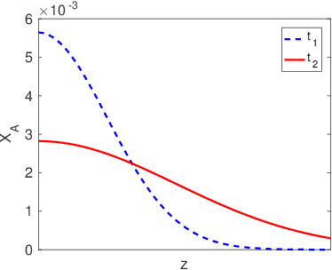
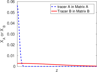
- Estimate the ratio
- Now suppose we measure the self diffusion coefficients of A and B. Performing measurements at the same time and temperature gives the concentration profiles shown in the figure above to the right. Which element (A or B) do you expect has the highest melting temperature, and why?
- Now we'll make a diffusion couple with element A on the right half and element B on the left half. Assume that A and B are miscible at the diffusion temperature, and form a one phase alloy. Mark up the following diagram as directed on the next page:
- Put an arrow labeled 'M' on the diagram indicating the direction that inert markers placed originally at the interface will move.
- Put an arrow labeled 'V' on the diagram indicating the the net vacancy flux due to diffusion in the sample.
- Put a 'C' on the region of the sample where you expect vacancies to be created, and a 'D' on the sample where you expect vacancies to be destroyed, assuming that the total vacancy concentration must remain at equilibrium.
- Two edge dislocations are also indicated in the diagram. Place arrows on top of each dislocation to illustrate he directions you expect these dislocations to move in order to create or destroy the vacancies from part iii.
Stress and Strain
13.0.0.10
A tensile stress, , is applied to a single crystal of zinc, which has an HCP structure. The close packed planes of atoms (the slip plane for an HCP material) is oriented with its surface normal in the plane of the paper, inclined to the tensile axis by an angle as shown below, with . Assume that the critical resolved shear stress for motion of the dislocation is 50 MPa (5x10 Pa). The shear modulus of Zn is 43 GPa (4.3x10 Pa) and its atomic radius is 0.13 nm.

- Is this an edge dislocation, a screw dislocation, or a mixed dislocation, and how do you know?
- Put an arrow on the drawing above to indicate the direction in which the dislocation moves under an applied tensile stress.
- Calculate the tensile yield stress for this sample.
- Suppose that the slip plane is oriented so that is still in the plane of the paper, but that is increased to . Will the yield stress increase, decrease or stay the same.
- Suppose that the dislocation is impeded by pinning points (precipitates, for example), that are uniformly spaced and separated by 1 m (10 m). The resolved shear stress is determined by the stress required to move the dislocation around these pinning points. Use the information given in this problem to determine the energy per length of the dislocation. Compare this to the expressions given for the energies of edge and screw dislocations to see if it makes sense.
Dislocation Structure
13.0.0.11
A right handed screw dislocation initially located in the middle of the front face of the sample shown below moves toward the back of the sample in response to an applied shear stress on the sample.
- Sketch the shape of the sample after the dislocation has propagated halfway through the sample, and again when it has propagated all the way through the sample. Use arrows to specify the shear force that is being applied.
- Repeat part a for a left-handed screw dislocation.
13.0.0.12
Draw an edge dislocation and on the same figure dot in the positions of the atoms after the dislocation has shifted by
13.0.0.13
How can two edge dislocations with opposite Burgers vectors meet to form a row of vacancies? How can they meet to form a row of interstitials? Draw pictures of both situations.
13.0.0.14
Given a crystal containing a dislocation loop as shown in the following figure:
Let the loop be moved (at constant radius) toward a corner until three-fourths of the loop runs out of the crystal. This leaves a loop segment that goes in one face and comes out the orthogonal face. Sketch the resultant shape of the crystal, both above and below the slip plane.
13.0.0.15
Given a loop with a Burger’s vector that is perpendicular everywhere to the dislocation line, determine the resulting surface morphology after the loop propagates out of the crystal. Assume that the loop moves only by glide.
13.0.0.16
Show that it is impossible to make a dislocation loop all of whose segments are pure screw dislocations, but that it is possible with edge dislocations. For the case of the pure edge dislocation loop, describe the orientation of the extra half plane with respect to the dislocation loop.
13.0.0.17
Draw the compressive and tensile regions surrounding an edge dislocation.
13.0.0.18
Consider the dislocation loop shown below:
- Circle the drawing below that corresponds to the shape of the material after the dislocation has expanded and moved out outside the crystal.
- Indicate in the spaces below the locations (a, b, c, or d) where the dislocation has the following characteristics:
- It is a right handed screw dislocation:_____
- It is a left handed screw dislocation:_____
- It is an edge dislocation with the extra half plane above the plane of the loop:_____
- It is an edge dislocation with the extra half plane below the plane of the loop:_____
- Add arrows to the illustration of the dislocation loop to show the orientation of the shear stress that will most efficiently cause the dislocation to loop to grow.
Dislocation Interactions
13.0.0.19
If edge dislocations with opposite signs of the Burger’s vectors meet, does the energy of the crystal increase or decrease? Defend your answer.
13.0.0.20
A nanowire is grown such that it is free of dislocations. Why would the stress required to deform the nanowire be larger than a bulk material?
13.0.0.21
If an anisotropic alloy system has a nearly zero dislocation line tension, would you expect the precipitate spacing to have a large effect on the yield stress of the alloy? Explain your reasoning
13.0.0.22
Given an edge dislocation in a crystal, whose top two-thirds is under a compressive stress acting along the glide plane (see figure below):
- If diffusion occurs, which way will thee dislocation move? Explain why and tell where the atoms go that leave the dislocation.
- Derive an equation relating the stress, to and the force tending to make the dislocation move in the vertical plane.
- If the edge dislocation is replaced by a screw dislocation, which which way will the dislocation tend to move?
13.0.0.23
Construct a plot of the interaction energy vs. dislocation separation distance for two identical parallel edge dislocations that continue to lie one above the other as climb occurs. Justify your plot qualitatively by explaining how the strain energy changes with vertical separation.
13.0.0.24
Repeat the previous problem for edge dislocations of opposite sign.
13.0.0.25
On the following sketch of a dislocation, indicate the direction that it must move in order for vacancies to be created.
13.0.0.26
Consider an isolated right-handed screw dislocation. Suppose a shear force is applied parallel to the dislocation line, as illustrated below.

- What is the direction of the force, , that is applied to the dislocation as a result of the applied stress.
- Suppose the screw dislocation is replaced by a dislocation loop with the same Burgers vector as the dislocation from part a, as shown below. Use arrows to indicate the direction at different points along the dislocation loop. (The direction of has already been indicated at the right edge of the dislocation).
- Describe how the magnitude of changes (if at all) for different locations along the dislocation loop.
- What to you expect to happen to the dislocation loop if you remove the external applied stress (will the loop grow, shrink or stay the same size)?
- Suppose the straight screw dislocation from is pinned by obstacles that are separated by a distance , as illustrated in the following figure. Sketch the shape of the dislocation for an applied shear stress that is just large enough for dislocation to pass around the obstacles.
- What do you expect to happen to the critical resolved shear stress of the material if is decreased by a factor of 2. (Will the critical resolved shear stress increase, decrease or stay the same).
Interfacial Thermodynamics
13.0.0.27
Consider the following:
- Is the molar latent heat positive or negative?
- Is the melting temperature , for a very small particle greater to or less than the equilibrium value of for a bulk material?
- Must this always be the case?
- For metals, what is the typical value of for which a change in melting temperature of 10K is observed. What about a change of 1K?
13.0.0.28
The molar enthalpy of a phase varies with temperature as
where is the molar heat capacity. Given this, at what temperature is the latent heat appearing in expression for the melting point reduction evaluated?
13.0.0.29
Consider the case of a pure liquid spherical droplet embedded in a pure solid. Create a graphical construction plotting the temperature dependence of the free energy of the solid and liquid phases(similar to Figure
5.11) for this case, and use it to determine if the melting point above or below the bulk melting temperature.
13.0.0.30
Consider the Co-Cu phase diagram shown below:
- Plot the equilibrium activity of Cobalt as a function of composition across the entire phase diagram at 900ºC.
- From the phase diagram, estimate the solubility limit of Co in Cu at 900 C. Suppose the interfacial free energy for the Cu/Co interface is . For what radius of a Co precipitate will this solubility limit be increased by 10%?
Surface and Interface Structure
13.0.0.31
Look up values for heats of sublimation for any of the materials in Table 6.1 that have close-packed crystal structures (FCC or HCP). Compare the estimated values of the surface free energy that you obtain from these heats of sublimation to the tabulated values in Table 6.1.
13.0.0.32
Determine the equilibrium shape of a crystal. This should be done using a computer and your favorite program or language (most likely MATLAB). The equation of a straight line in polar coordinates drawn from the origin of the polar coordinate system is
, where
locate the points on the line,
is the perpendicular distance from the origin to the line and
is the angle between the perpendicular to the line and the x-axis (see Figure
13.3).
- Determine the equilibrium shape of a crystal where the surface energy is given by J/m (independent of ).
- Determine the equilibrium shape of a crystal where the surface energy is given by J/m ( in radians). Are there any corners on the equilibrium shape?
- Determine the equilibrium shape of a crystal where the surface energy is given by J/m . Are there any corners on the equilibrium shape?
- Determine the equilibrium shape of a crystal where the surface energy is given by J/m . Are there any corners on the equilibrium shape? How is the shape shown in (c) different from that in (d), and why (argue on the basis of the physics of the problem)?
As a headstart on this problem, here's a MATLAB script that generates polar plots of the
as defined in the problem:
close all
A=[0,0.05,0.07,0.6];  % these are the 4 values of A defined in the problem
% define a function where the radius d is the surface energy and alpha
% is the angle
d=@(A,alpha) 1+A*cos(4*alpha);
figure
for k=1:4
    alpha=linspace(0,2*pi,200);
    subplot(2,2,k)  % this makes a 2 by 2 grid of plots
    polar(alpha,d(A(k),alpha),'r-');  % poloar is the command to make a polar plot
    title(['A=' num2str(A(k))],'fontsize',20)  % label each subplot
end
% adjust the print command as necessary to change the format, filename,
% etc.
print(gcf,'../figures/matlabwulffenergy.eps', '-depsc2') % save the eps file
This generates the following polar plots for the four different functions that are given (with defined so that ).
13.0.0.33
Assume a simple cubic crystal structure with nearest neighbor interactions. Calculate the ratio of the surface energies for the {110} and {100} surfaces.
13.0.0.34
The octahedral particles of FCC golds shown below were created by controlling the growth rates of the different crystal facets. For these crystals, were the growth rates fastest in the directions or in the directions? Provide a brief explanation of your answer.
13.0.0.35
The relationship between the the interfacial energy between and phases and the pressure difference across a curved interface is obtained from the following expression:
- Use this expression to obtain the pressure difference between a cylinder of phase with a radius and a surrounding phase.
- Repeat the calculation for a cube where the length of each side is . Assume that the surface energy of each of the cube faces is the same.
Wetting and Contact Angles
13.0.0.36
Consider the an oil droplet that forms on the surface of water, as shown schematically in the following Figure:
Determine and if the air/water interfacial free energy is 72 mJ/m , the air/oil interfacial free energy is 30 mJ/m and the oil/water interfacial free energy is 50 mJ/m .
13.0.0.37
Suppose a, hemispherical liquid Au droplet with a radius of curvature of is in contact with solid Si cylinder with the same radius as shown below. Derive a relationship between the three interfacial energies that must be valid in order for the equilibrium shape of the Au/Si interface to be flat, as drawn in the picture.
Grain Boundaries
13.0.0.38
The surface energy of the interface between nickel and its vapor is 1.580 J/m at 1100K. The average dihedral angle measured for grain boundaries intersecting the free surface is 168 . Thoria dispersed nickel alloys are made by dispersing fine particles of ThO in nickel powder and consolidating the aggregate. The particles are left at the grain boundaries in the nickel matrix. Prolonged heating at elevated temperatures gives the particles their equilibrium shape. The average dihedral angle measured inside the particle is 145 . Estimate the interfacial energy of the thoria-nickel interface. Assume the interfacial energies are isotropic.
13.0.0.39
Consider a gold line deposited on a silicon substrate. The grain boundaries run laterally completely across the line, giving a “bamboo” structure as shown in the figure below. The grain boundary energy of gold at 600K is 0.42 J/m and the surface energy is 1.44 J/m . Assume all the interfacial energies are isotropic.
- Compute the dihedral angle ( in the diagram above) where a grain boundary meets the external surface.
- Find the critical grain boundary spacing for which the equilibrium grain shape produces a hole in the film, assuming . Note that for a spherical cap, h and are related to each other by the following expression: .
13.0.0.40
Why does the velocity of a grain boundary depend on temperature? Assume that the driving force for grain boundary motion is independent of temperature.
13.0.0.41
Consider the following junction between three grains. Suppose that the grain boundary free energy between grains 1 and 2, and between 1 and 3, is 0.5 J/m . What is the grain boundary energy between grains 2 and 3?
13.0.0.42
Consider the following image from the grain growth simulation:
- The boundary marked with an 'X' separates grains 1 and 2. Do you expect this boundary to move toward grain 1 or grain 2 during the process of grain growth?
- Suppose that the interface marked above is the cross section through a grain boundary in aluminum, and that this section of the grain boundary has a spherical shape with a radius of curvature of m. Assuming a grain boundary energy of 0.25 J/m , calculate the chemical potential difference, between Al atoms on the '1' and '2' sides of the grain boundary.
- On the schematic below, indicate which grain is grain 1 and which one is grain 2.
- Suppose is the rate at which Al atoms hop from grain 1 to grain 2, and is the rate at which atoms hop from grain 2 to grain 1. Calculate the ratio, at K.
Transformation Kinetics
13.0.0.43
Does the time to 50% transformed increase or decrease with an increase in nucleation rate? Defend your answer without using any equations.
Interphase Interfaces
13.0.0.44
Consider a material with the orientational dependence of the surface energy shown in each of the 3 plots below. For each of these three materials, sketch the equilibrium shape that you would expect to obtain. On each drawing, indicate any interfaces that you expect to be coherent.
13.0.0.45
Consider the shapes of the particles in the simulations below of misfitting particles in an elastically anisotropic system. The left column is the entire system, whereas the right column is a magnification of a small region of the figure in the left column. These are snapshots taken as function of time while the particles are growing. Are these cuboidal shapes due to elastic stress, an anisotropic interfacial energy, or both?
13.0.0.46
Explain the structure and energies of coherent, semicoherent and incoherent interfaces, paying particular attention to the role of orientation relationships and misfit.
13.0.0.47
Explain why fully coherent precipitates tend to lose coherency as they grow.
13.0.0.48
Why do very small precipitates tend to have coherent interfaces?
13.0.0.49
A thin film of Zn with an HCP crystal structure is deposited on a Ni FCC substrate with a {111} orientation. Which plane of the HCP crystal would you expect to contact the {111} Ni surface?
13.0.0.50
Given an example of an interface between two crystals that that displays a very large change in free energy with a change in the orientation of the interface.
13.0.0.51
Consider an FCC metal (metal A) with a surface energy of 1 An HCP metal (metal B) with a surface energy of 0.7 is deposited onto the {111} surface of metal A. Assume that the atomic diameter of the HCP metal is 3% larger than the atomic diameter of the FCC metal, and that the chemical component of the interfacial energy between the two metals is 0.2
- For B layers that are sufficiently thin, do you expect that a coherent interface will form between the A and B materials? Justify your answer.
- How do you expect the interface between the A and B metals to change as the thickness of the B layer increases?
- Do you expect thick films to remain continuous, or will isolated drops of B be formed on the surface. Describe any assumptions that you make.
13.0.0.52
Consider the vacancy shown below, for a simulation of 'red' and 'blue' atoms that are undergoing phase separation. Is the vacancy more likely to move to the right or to the left? Justify your answer.
13.0.0.53
Consider the tilt boundary shown in the image to the left. On the axes on the right, sketch the relationship between the grain boundary free energy and the tilt angle that you expect to observe for values of theta between 0 and 10 .
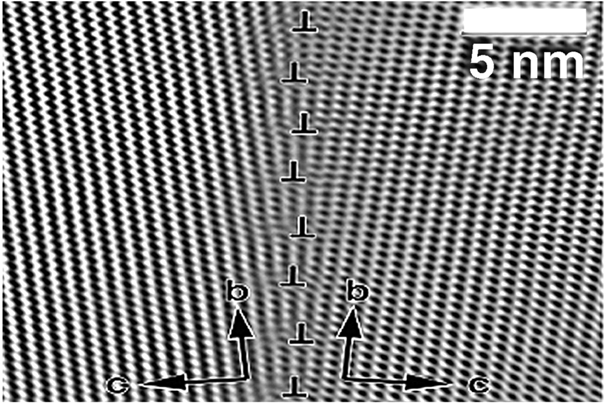
(5
13.0.0.54
Suppose you need to apply a coating to a surface, and you want the coating to spread as a smooth uniform film for all thicknesses. You have a choice of three different coatings, which have the thickness-dependent free energies shown below. Which material to you choose, and why?
14 316-1 Simulation Exercise: Monte Carlo Simulation of Decomposition in a Binary Alloy
14.1 Background
14.1.1 Scientific problem
We want to analyze the thermodynamic evolution of a A-B alloy by simulation. We assume that this system has the phase diagram presented in Figure
14.1. In this figure we see that for temperatures lower than
, the A-B alloy decomposes in two phases
and
with equilibrium concentrations
and
. The experiment that we want to model involves the following steps:
- We mix together the same number of moles of elements A and B to obtain a homogeneous alloy at some temperature above .
- The temperature is reduced to .
- The temperature is held fixed at , and the system evolves to form two different phases, with compositions and .
14.1.2 Atomistic Monte Carlo Model
In this section, we introduce the Atomistic Monte Carlo model that we will use to model the decomposition of the A-B alloy.
14.1.3 Atomistic model
In this model, we suppose that the two elements (A and B) have the same lattice structure. This lattice is represented by a matrix with periodic boundary conditions on its edges (see Figure
14.2). In 2 dimensions the left edge is connected to the right edge and the upper edge is connected to the lower edge. We reproduce the system evolution at the atomistic level: vacancies present in the lattice migrate from site to site by exchanging their position with their first nearest neighbors. The successive displacements of vacancies make the system evolve toward its equilibrium state.
14.1.4 Monte Carlo model
The thermodynamic evolution of the alloy is modeled with a Monte Carlo process. The principle of Monte Carlo simulations is to model the A-B alloy evolution in a statistic way. To understand this model we can consider individual jumps of a vacancy into one of the nearest neighbor positions. Within a certain specified time step, , these different possible jumps occur with a probability where is an index that indicates which direction the vacancy will move. In a simple cubic lattice, for example, = 6, and the 6 values of correspond to jumps in the positive and negative x, y and z directions. The sum over all possible jump probabilities in the statistical time must sum to 1:
To figure out which direction the vacancy moves, we draw a random number between 0 and 1. The jump performed by the system during the time is the one such that the following condition holds:
Probabilities of transitions are related to the energetic barrier associated with vacancy motion, which we refer to as . Because vacancy hopping is a thermally activated process, we can use an Arrhenius rate expression:
where is a constant, is Boltzmann's constant and is the temperature of the system.
The energy barrier is the difference between the maximum energy of the system during the jump (the position of the migrating atom at this maximum energy is called the saddle point) and the energy of the system before the jump.
Here the superscript
refers to 'Saddle Point' and
means 'initial', as shown in Figure
14.3.
14.1.5 Energetic model
To compute the energy barriers of the different possible jumps , we have to use an energetic model. In Monte Carlo simulations, we usually use an Ising model or Broken bond model. In this energetic model, we assume that the total energy of the system is equal to the sum of interaction energies between the different elements (atoms of type A and B and vacancies V) placed on the lattice sites.
With this energetic model, the migration barrier of an exchange between an element and the vacancy becomes:
where are interaction energies between the atom migrating and its neighbors at the saddle point, are interaction energies between the atom migrating and its neighbors before the jump and are interaction energies between the vacancy and its neighbors before the jump. The indices i, j and k indicate the following neighbors:
|
Index
|
Meaning
|
|
i
|
nearest neighbors of the migrating atom before the jump
|
|
j
|
nearest neighbors of the vacancy before the jump
|
|
k
|
nearest neighbors of migrating atom at the saddle point
|
In theory, the range of interaction distances between elements are unlimited. In practice, we usually restrict these interactions to first and sometimes second nearest neighbors.
For example, the system presented in figure
14.4 has:
- 3 A-V interactions
- 1 B-V interaction
- 3 A-B interactions
- 9 A-A interactions
- 12 B-B interactions
Therefore,
. If we suppose that the vacancy exchange its position with the B atom on its left side, the configuration of the system at the saddle point is the one presented in figure
14.5.
In this configuration, the system has:
- 2 B-B interactions at the saddle point
- 2 A-B ineractions at the saddle point
- 3 A-B interactions
- 9 A-A interactions
- 9 B-B interactions
so . The migration barrier of this jump is therefore:
14.1.6 Modeling of scientific problem
Here we assume that the two elements A and B have the same simple cubic lattice. We model the A-B alloy as a matrix in 2D with rows and columns and with periodic boundary conditions on its edges. To simplify the problem, we introduce only one vacancy in the lattice (so 1 vacancy for sites), initially located in the middle of the matrix. As we only interest ourselves to the thermodynamic evolution of the system (and not to its kinetic evolution), we assume that the alloy evolves with normalized time steps of 1 until a maximum time . At each time step, the vacancy exchanges its position with one of its neighbors.
To simplify the energetic model we suppose that the sum of interaction energies between the atom migrating and its neighbors at the saddle point is a constant equal to . In addition, we suppose that . The only interaction which can be different from zero is thus .
The free enthalpy of the alloy is expressed by
with the ordering energy of the alloy and the configurational entropy of mixing of the alloy given by :
For a symmetrical miscibility gap, the ordering energy is
where is the critical temperature of the miscibility gap ( in this study). In broken bond models with only first nearest neighbors interactions we have:
where is the number of first nearest neighbors for a given site.
14.1.7 Algorithmic scheme : Translation of problem in algorithm
In this section we translate the problem described previously in an algorithm scheme. As we are modeling an evolution according to time, our code will contain an initial state and an incremental loop on time which will start from the initial time () and finish at a final time (). During the time loop (for example between time and ), the code will repeat the same operations which will make the matrix go from the configuration at to the one at . In this code we suggest that the system evolves with the following steps in the time loop:
- Evolution of time from and
- Computation of jump frequencies of all possible jumps
- Drawing of a random number and choice of a jump according to Eq. 14.2.
- Completion of chosen jump: exchange of position between vacancy and nearest neighbor chosen.
14.2 Exercise
Random walks
In this first work, we model the evolution of the system if the equilibrium configuration of the alloy is an homogenized state. As we only interest ourselves to the thermodynamic evolution of the system (and not to its kinetic evolution), we assume that the alloy evolves with normalized time steps of 1 until a maximum time . At each time step, the vacancy exchanges its position with one of its neighbors. The vacancy can exchange its position with all its first nearest neighbors (and only its first nearest neighbors). The difference is that in this section we suppose that all exchanges have the same jump frequency . This is called a“ random walk”.
14.2.1 Preliminary work
- Consider a vacancy located on the lattice site as in Figure (14.6). In this figure, identify the first nearest neighbors of the vacancy by numbers and give the coordinates of these neighbors according to .
- Suppose that all exchanges of the vacancy with its first nearest neighbors have the same jump frequency. Using equation (14.1), give the probability of a given jump .
14.2.2 Simulation
- Create a folder for this MATLAB project. Open a new script in Matlab and save it in your folder as “part1.m”.
- We first write the initial state of the system in the file part1.m. Save the matrix given in the file called 'matini.mat' available from the following link:
https://www.dropbox.com/s/y4o2q3v53ffwinw/matini.mat?dl=0
Load this matrix in part1.m as “matrix”. Define and as the number of rows and column respectively of matrix. In this matrix, elements A are identified by a number 1 and elements B are identified by a number 2. Place a vacancy (identified by a 0) in the middle of the matrix:
- define in part1.m the coordinates (where is the row and the column of the vacancy position) as the coordinates at the middle of the matrix.
- Place a 0 in the matrix at the appropriate coordinates .
Initialize time to 0.
- If the matrix has the configuration of figure 14.6, what does the matrix in Matlab look like (with the numbers)? (Include a printout of the matrix).
- Create a loop on time where time evolves by steps of 1 as long as remains lower than . Place . We now have the part 1 in the algorithm (see section 14.1.7). Attach part1.m that includes all of the steps so far.
- We now have to create the next part of the algorithm: the computation of the jump frequency of all possible jumps. (Remark: in this random walk program, this part could be placed outside of the time loop since all jumps have the same frequency. However, we include it in the time loop to prepare the second part of the problem where we will have to compute the according to the environment). In the program, we call the vector such that is the jump frequency of the exchange . Use a “for” loop to compute the values of the different components.
- We now have to choose a jump amount the different possibilities. For this, we suggest the MATLAB code shown below - just a single line that results in a random integer between 1 and 4:
njump = randi([1 4], 1, 1)
Run this command 5 times and write down the numbers you get for njump. Does this make sense?
- For the chosen jump, identify in your code by the coordinates of the corresponding nearest neighbor according to . For this, we suggest you to define a matrix () of the different possible evolutions (for example or ) and to write according to and the column of the matrix corresponding to the jump.
- We use periodic boundary conditions in this model (see part 14.1.3). For a site , verify that the following function enables to apply boundary conditions presented in figure (14.2) For this, respond to the following questions: what is the value of returned by this function if the in input is between 1 and ? equal to 0? equal to ? Apply this function to and .
- Exchange types of elements corresponding to the vacancy an the neighbor migrating in the matrix.
- Update the vacancy coordinates to its new site.
- In this random walk model, what is the equilibrium state of the system? (Help: the fact that all the are equal induces that the migration barriers for all possible jumps are equal. From equation (14.6) it induces that all saddle point interactions and are equal, all atom-atom interations are equal and . What is thus the value of the ordering energy in equation (14.10)? And the value of ? So at any temperature, what is the equilibrium state of the system?)
- Test: Replace the initial matrix by a matrix of same size with all A atoms on the half left side and all B elements on the half right side. Print an image of this initial matrix. Make the code run until . What do you observe? Print an image of the final matrix.
14.2.3 Introduction of alloy thermodynamic properties
We now have to introduce the alloy thermodynamic properties in the code. We thus have to compute the jump frequency of possible exchanges between the vacancy and its neighbors according to the alloy thermodynamic properties.
- We recall here that . Express according to the ordering energy and then to the critical temperature . Give a numerical value of in eV if .
- We analyze the migration barrier of an exchange between a vacancy V and one of its nearest neighbors . We note the number of first nearest neighbors of type A and the number of first nearest neighbors of type B. How many first nearest neighbors does X have (we do not count the vacancy)? Express equation (14.6) according to , and and . Using that and that , simplify the equation obtained if X is an element A. Same question if X is an element B. We observe from these calculations that, to compute the migration barrier of a jump, we need to know the type of the element of the exchange (so the type of ) and the type of all first nearest neighbors (to compute and ).
- For a given vacancy position, we want to compute the jump frequency of the jump (so ). We note the vacancy neighbor corresponding to this jump. We start by computing and (the number of first nearest neighbors of type A and B). We note the position of and the coordinates of first nearest neighbor ( goes from 1 to 3, the vacancy position is excluded from these nearest neighbors). We write where is the column of the matrix of relative position of compared to . Graph 14.7 gives the position of neighbors compared to the vacancy.
0For each of these jumps, associate the matrix of the relative position of first nearest neighbors.
- Inside the loop to compute coefficients write the following steps:
- define by the vacancy neighbor corresponding to (use the matrix). Apply periodic conditions to .
- Initialize and to zero. Compute and of the exchange by analyzing the type of element on all sites. To define the matrix corresponding to the jump, you can distinguish the different cases with if-statements or you can use a structure with all the matrices and load the one corresponding to the jump. Don't forget to apply boundary conditions to .
- Express the migration barrier of each jump depending on the type of the neighbor (located on ) and and . Compute the jump frequency associated to this migration barrier (place the temperature to an arbitrary value-don't forget to define in your code).
- Normalize the vector to 1 so that the sum of is equal to 1.
- Analytic calculation: Suppose that for a given position, the vacancy can exchange it's position with either of 2 different A atoms. One on them is in a local configuration with NB=0 (the jump frequency of this exchange is noted ) and the other one is in a local configuration with NB=3 (the jump frequency of this exchange is noted ). Compute for T=100K and for T=2000K. Explain why these ratios are consistent with the alloy phase diagram.
- Place the temperature to 100K. Run the simulation until . What do you observe?
Nomenclature
- $C_{0}$
- Overall concentration of atoms
- $C_{i}$
- Concentration of component i
- $D_{i}$
- Intrinsic diffusion coefficient for component i (m$^{2}$/s)
- $D_{i}^{*}$
- Tracer diffusion coefficient for component i (m$^{2}$/s)
- $E$
- Energy (J)
- $E_{s}$
- Dislocation Energy (J)
- $F_{s}$
- Force per unit length acting on a dislocation (N)
- $F_{s}^{\tau}$
- Stress-induced force per unit length acting on a dislocation (N/m)
- $F_{s}^{r}$
- Curvature-induced force per unit length acting on a dislocation (N/m)
- $G$
- Shear modulus (Pa)
- $H_{i}$
- Henry' law coefficient for component i (dimensionless)
- $J_{i}$
- Diffusive flux of component i with respect to a cooridnate system fixed to the lattice planes (atoms/m$^{2}$/s)
- $J_{i}^{'}$
- Diffusive flux of component i with respect to a cooridnate system fixed to the external dimensions of the sample (atoms/m$^{2}$/s)
- $L_{m}$
- Molar heat of sublimation (Joules)
- $M_{i}$
- Mobility of component i (units of velocity/force)
- $R$
- Gas constant (8.314 J/mole$\cdot$ K)
- $S_{m}^{L}$
- Molar entropy of the liquid phase
- $S_{m}^{S}$
- Molar entropy of the critical nucleus
- $T$
- Absolute temperature (K)
- $T_{s}$
- Dislocation line tension (N or J/m)
- $V$
- Volume (m$^{3}$)
- $V_{m}^{S}$
- Molar volume of the solid phase
- $\ell_{i}^{D}$
- Diffusion length for component i (m)
- $\gamma_{\alpha\beta}$
- Interfacial free energy between $\alpha$ and $\beta$ phases (J/m$^{2}$)
- $\hat{s}$
- Unit vector directed along a dislocation core (dimensionless)
- $\mu_{i}$
- Chemical potential of component i (J/mole)
- $\sigma$
- Tensile stress (Pa)
- $\tau$
- Shear stress (Pa)
- $\tau_{crss}$
- Critical resolved shear stress (Pa)
- $\tau_{crss}^0$
- critical resloved shear stress in the absence of dislocations
- $\tau_{rss}$
- Resolved shear stress (Pa)
- $\tilde{D}$
- Interdiffusion coefficient (m$^{2}$/s)
- $\vec{b}$
- Burgers vector (m)
- $\vec{n}_{d}$
- Vector cross product of $\vec{s}$ and $\vec{b}$ (m)
- $a_{i}$
- Activity coeffiienct for component i (dimensionless)
- $b$
- Magnitude of $\vec{b}$ (m)
- $e_{xy}$
- Shear strain in the x-y plane
- $k_{B}$
- Boltzmann's constant (1.38x10$^{-23}$ J/K)
- $n_{i}$
- Total number of atoms of component i.
- $r$
- Particle radius (m)
- $v_{\ell}$
- Velocity of the lattice planes with respect to a laboratory coordinate system (m/s)
- F
- Helmholtz free energy
- G
- Gibbs free energy
Index
- Burgers circuit: 1
- Burgers vector: 1
- Climb (of a dislocation): 1
- Contact angle: 1
- Critical resolved shear stress: 1
- limiting value in the absence of dislocations: 1
- Cross slip: 1
- Diffusion equation: 1
- Dislocation
- Dislocation density: 1
- Dislocations
- cross product: 1
- Screw: 1
- Sense vector: 1
- Edge dislocation: 1
- error function: 1
- Fick's first law: 1
- Frank-Read source: 1
- Gibbs free energy: 1
- Glide: 1
- Glide plane: 1
- Hall-Petch relationship: 1
- Heat of sublimation: 1
- Helmholtz free energy: 1
- Henry's law: 1
- Henry's law coefficient: 1
- Heteroepitaxy: 1
- Interdiffusion coefficient: 1
- Intrinsic diffusion coefficient: 1
- Johnson-Mehl-Avrami-Kolmogorov (JMAK) equation: 1
- Lagrange Multipliers: 1
- Laplace pressure equation: 1
- Laplace-Young equation: 1
- MATLAB
- fsolve: 1
- Function plot: 1
- loading and plotting data from .mat file: 1
- polar plot: 1
- setting plotting defaults: 1
- Vacancy diffusion simulation: 1
- Wulff Construction: 1
- Miller indices: 1
- mobility coefficient: 1
- Partial wetting: 1
- Resolved shear stress: 1
- Screw Dislocations: 1
- Sense vector: 1
- Slip Plane: 1
- Thin Film Growth: 1
- Three phase contact lines: 1
- Tilt boundary: 1
- Twin boundaries: 1
- Twin boundary: 1
- Twist boundary: 1
- Wulff construction: 1
15 316-1 Labs
15.1 Laboratory 1: Diffusion in Substitutional Cu-Ni Alloys
15.1.1 Objectives
- To observe diffusion in a Cu-Ni diffusion couple.
- To determine if these observations are consistent with a composition-dependent interdiffusion coefficient, expected for diffusion in substitutional alloys.
- To begin to model the diffusion process using MATLAB.
15.1.2 Introduction
In the case of pack-carburization, we were able to make the assumption that diffusivity of carbon in iron was independent of composition. For substitutional alloys, this is not the case. The interdiffusion coefficient in this case is composition dependent and related to the intrinsic diffusion coefficients as follows:
In addition, in situations where and differ from one another, there will be a net vacancy flux in the material, giving rise to the motion of an inert set of markers that can be observed experimentally.
15.1.3 Samples
Samples have been prepared using two techniques:
- electroplating of nickel layers onto copper, and
- welding Ni-Cu sandwich layers.
In both cases, Mo wires were placed at the interface, to mark the position of the original interface; however in the case of the electroplated samples, these wires sometimes shifted away from the surface during plating. After electroplating/ welding, the samples were sealed in evacuated quartz tubes to prevent oxidation, and annealed at 1000°C for 4, 16, and 72 hours.
15.1.3.1 Laboratory Procedure
Refer to the class notes in addition to the paper describing the background and history of the Kirkendall effect [
6]. Look at the Cu-Ni samples (annealed at 4, 16 and 72 hours at 1000 °C) under the optical microscope. Note that there are two types of sample: 1) copper strips wound with Mo wire which were nickel-electroplated and 2) a welded "sandwich" of nickel with outer copper layers and rolled molybdenum "marker wires" at the interface. Note that in (1) the Mo was not secured to the copper strip well-enough to mark the original interface (this will be obvious in your observations). In (2) you will find enough pairs of wires that are nearly across from each other to measure the distance between markers as a function of time at elevated temperature. (Unfortunately, the weld broke on the unannealed (time = 0) samples; but you should be able to assess the three remaining samples quantitatively or at least semi-quantitatively. Include these measurements with your other observations, as well as a discussion of what you expected. Discuss whether or not your observations and measurements are consistent with the Kirkendall effect. In future exercises we will be comparing these diffusion profiles to what we would expect from published values of the relevant diffusion coefficients. For now document your in-class observations, including well labeled sketches and micrographs.
15.2 Laboratory 2: Recovery, Recrystallization and Grain Growth in Cold Worked 70/30 Brass
15.2.1 Objectives
To observe the phenomena of recovery, recrystallization and grain growth. To understand the effect of processing on microstructure, specifically the effect of amount of cold-work on recrystallization and final grain size. To understand the time dependence of grain growth. To understand the predictions of the Hall-Petch relationship.
15.2.2 General Procedure: Week 1
You will be provided with brass (70%Cu, 30% Zn) that has been heated to 700° C for six hours, from the as-received state and then rolled to reductions of ~ 15% and ~ 30%, as well as some brass that has not yet been rolled. Your groups will cold-roll samples to similar reductions for the next group. The specified amount of cold-work will be introduced using the rolling mill.
- Measure the thickness and the Rockwell hardness of your as-received and rolled samples. Choose an appropriate Rockwell scale over which you can anticipate measuring your sample after it is rolled – then subsequently annealed. Always check to make sure the load and indenter size correspond to the correct scale. Use a standard to check the tester.
- As a group, roll two samples, using the rolling mill, one to a reduction of ~ 30-40%, a second to a lesser reduction, e.g. 15-20%. Anticipate the target thickness before you begin rolling. Calculate target thicknesses for each reduction, assuming width does not change with rolling. Percent reduction (or percent coldwork) is defined as:
which may be re-written for this lab:
where is the starting thickness and is the final thickness. Set aside for the next group.
- Re-measure hardness after rolling. (Make sure to measure a flat region. The sample should not deflect when the indenter is applied.)
- Section the rolled samples into about 8 pieces (~ 1cm long). Note that we will be interested in observing the transverse sections, defined in the figure below. Set aside a time = 0 sample; each of the other 1 cm long “coupons” will be annealed at a specified time at the temperature assigned to your group
- Record the temperature assigned to your group. T=___ degrees C.
- samples that have been annealed from 2 minutes, 8 minutes, 32 minutes….up to a week. You will be measuring and recording Rockwell hardness on each of these samples, then mounting them for polishing and etching.
- After reserving the time = 0 sample, place the remaining samples in the furnace assigned to your lab group. (All samples of both reductions, except t=0, should be annealed at the SAME TEMPERATURE
***Suggest (the entire group’s) annealing conditions by reviewing information available in the Metals Handbook, and by discussion with your lab mates & instructor. You want to achieve conditions under which you will observe partial to total recrystallization. Consider how you will need to vary the conditions to test the Johnson-Avrami-Mehl equation.
15.2.2.1 General Procedure: Week 2
- Make sure you have measured the Rockwell hardness of each annealed sample. Note that you should try to take all your hardness readings on the same scale.
- Mount transverse cross-sections of each of the annealed samples, along with an unannealed piece in an acrylic mount for polishing. Follow the instructions for the auto-polisher. Wash your sample carefully and ultrasonic between each step to avoid contaminating the wheels. (These are soft samples; it will be difficult to remove the scratches that are introduced by such contamination!)
- Etch to reveal grains. (Be careful; the different reductions and different temperatures of annealing may result in different etch rates.) Record a photomicrograph of each sample at an appropriate magnification.
- From your micrographs, calculate the volume fraction of recrystallized material, and the grain size of samples that are completely recrystallized.
- Measure the Vickers hardness of each sample (three indents, minimum, on each sample.)
15.2.3 In-Lab Questions DUE at the Beginning of Week 2:
Rolling, hardness testing and cutting will take some time. If you are waiting you may use time in lab to answer the following. Make sure you define all terms and cite sources:
- What equation describes the rate of grain growth?
- Refer to Chapter 3 of Shewmon and summarize the “Engineering Laws of Recrystallization” relevant to this experiment. (You may summarize all – then determine which you might be able to test vs. not able to test.)
- What equation describes the volume fraction of material recrystallized with time?
- How can the rate of recrystallization at a given temperature be determined?
- What is the Hall-Petch equation? Discuss the equation and any limitations.
15.2.4 Final Deliverable - Group PowerPoint Presentation
Your presentation will be judged on content, delivery (presentation style), neatness, completeness. You must submit a hardcopy of your presentation slides. Imagine you are presenting this to Prof. Voorhees and other MSE students who were not in lab; they are familiar with terms like grain size and hardness, but do not know the details of your sample preparation and what you are testing (i.e. which of the Engineering laws of Recrystallization you were able to test.) Length: 12 minutes. Each group member must participate.
Due: one week after completing in-class measurements.
- Refer to Chapter 3 of Shewmon; discuss whether or not the class data substantiates the “Engineering Laws of Recrystallization,” i.e. how do hardness, grain size, volume fraction of recrystallized material vary with the amount of cold-rolling, and time of anneal? Plot hardness (Rockwell is OK, here) as a function of annealing time for both reductions, including time = 0 values. Explain changes in hardness by comparison with micrographs.
- Estimate the recrystallization rate for your group’s annealing temperature: Rate = 1/(time for volume fraction transformed = 0.5).
Note: We will try to use the information from different groups to compare recrystallization as a function of temperature. If you have enough points (this is unlikely), you may be able to fit the Avrami (JMAK) equation:
- Make sure you use actual – not target reductions – when discussing your results. Double-check that the reduction is, for example, 40%, not 70%.
- For samples in which complete recrystallization was observed – does the Hall-Petch relationship hold? Assume that hardness is proportional to yield strength (see next page). The Hall Petch equation states that the yield stress, , is increases linearly with , where is the average grain size:
where and are constants for a given material. Note that you do not have to confine comparisons to a single recrystallization; use all the samples available that have recrystallized. (It tends not to be valid for very large or very small grains.)
- For completely recrystallized samples, is normal grain growth observed? Measure grain sizes for recrystallized material at a given reduction and determine the exponent for grain growth as a function of annealing time at a given temperature:
Solve to see if is greater than or equal to 2, as expected. Note that at the start of recrystallization, the grain size is infinitesimally small.
15.2.4.1 Heyn Procedure for counting lineal intercept length:[4]
- Estimate the average grain size by counting, on a micrograph, screen or the specimen itself, the number of grains intercepted by one or more straight lines sufficiently long to yield at least 50 intercepts. Select the magnification such that this can be done in a single field.
- Make counts on 3-5 blindly selected, widely separated fields.
- Use a factor of 1.5 to determine the average grain size from the lineal intercept length.
15.2.4.2 Hall–Petch determination:
- Measure Vickers hardness.
- Use hardness and grain size to determine if the Hall-Petch relationship holds true for your data. (Plot HV vs. )
- You can use Vickers hardness to calculate the Yield strength of brass. Assume 1/3 of the applied load in a Vickers Hardness test plastically deforms the sample and use the appropriate conversion factor () to convert to MPa:
Q – Are your values of yield strength within a reasonable range? Compare to typical values (Metals Handbook)
15.2.4.3 Empirical relationship between Rockwell B and Vickers hardness (kg/mm).
Note that it is best to measure the Vickers hardness directly. The following relationship between the Vickers hardness ( and Rockwell B hardness () is obtained from ASTM Standard E140 (table 4, Conversion data for Cartridge brass), Annual Book of ASTM Standards, volume 3.01, 1989:
15.3 Laboratory 3: Surface Energy and Contact Angles
15.3.1 Objectives
- To understand what aspects of liquid behavior are determined by surface and interfacial energies.
- To understand how contact angles are used to characterize material surfaces.
15.3.2 Introduction
The properties of solid surfaces are often probed by measuring the ability of liquids to spread over the surface of a material. The relevant property is the contact angle,
, illustrated in Figure
15.1a. If the droplet is small enough so that it is not affected by gravity, the radius of curvature,
, of the droplet is uniform, and shape of the droplet is a spherical cap,
i.e., the portion of a sphere that exists above a specified plane. The relationship between the droplet height,
, the basal radius of the droplet,
, and the contact angle in this situation is as follows:
At equilibrium, a horizontal force balance at the periphery of the object gives the following expression for the equilibrium contact angle,
and the relevant surface and interfacial energies (Figure
15.1b):
It is often useful to rewrite Eq.
15.8 in terms of the thermodynamic work of adhesion,
, which describes the energy required to remove the liquid from the solid surface, replacing the solid/liquid interface with a liquid/air interface and a air/solid interface (see Figure
15.2):
Here
is the solid surface free energy,
is the liquid surface free energy and
is the solid/liquid interfacial free energy. Note that for liquids, the surface tension and the surface free energy are identical to one another, so we refer to
as either the liquid surface tension or surface free energy.
Combination of Eqs.
15.8 and
15.9 gives the following:
Equation
15.10 indicates that we can know the quantitative interaction between the liquid and the solid if we are able to measure the liquid surface energy,
and the equilibrium contact angle,
. This purpose of this lab is to measure both of these quantities in some model systems and to show how these quantities can be easily modified. Before we do that, we need to talk about two important issues:
- The actual contact angle you will measure is almost certainly not going to be the equilibrium contact angle.
- Liquid surface energies are often measured by understanding the effect of gravity on a relatively small drop.
15.3.2.1 Non-equilibrium effects:
In reality, the situation is more complicated than is implied by Eq.
15.8, and the contact angles you will measure depend on a whole bunch of factors, in addition to the surface and interfacial energies. Factors like surface roughness and surface inhomogeneities on the nanometer scale cause the measured contact angles differ from the
, and to depend on the details of the way the experiment is done. When a droplet is originally applied to the materials surface and the droplet volume is increasing with time, the contact angle is referred to an advancing contact angle,
. The receding contact angle,
, corresponds to the opposite situation, where the droplet size is shrinking. The advancing contact angle is larger than
and the receding contact angle will be less than
:
Generally you'll want to report both advancing and receding angles in your work. The difference between and is an important parameter referred to as the contact angle hysteresis, and controls the tendency of droplets to stick to an inclined surface.
15.3.2.2 The Effect of Gravity and the Measurement of
We know from experience that Eq.
15.7 can't work for very large droplets. Eventually, gravity flattens the droplet and the drop height,
, no longer continues to increase as
gets larger and larger. This situation is as shown in the left part of Figure
15.3, where we show the behavior of small and large droplets sitting on a surface (sessile drops). The obvious question to ask here is 'how small is small'? and what controls the maximum value of
that can be obtained? The answer to this question is the capillary length,
, which can be viewed as the radius of the spherical droplet for which the Laplace pressure inside the drop (
is equal to the gravitational hydrostatic pressure at the bottom of the drop (
, where
is the gravitational acceleration and
is the liquid density). These pressures are equal to one another for
, where
is given by the following:
The capillary length determines the degree to which gravity distorts the droplet the droplet from a spherical cap, with no noticeable distortion observed for
. The measurement can done sessile drops like those in the left part of Figure
15.3, but it is generally more accurately done for the pendant drop geometry at the right of Figure
15.3. The pendant drop geometry is used in this laboratory. The software automatically measures the shape of the droplet and determines the capillary length from the shape, which is then converted to a surface energy using Eq.
15.3 and a known value of the liquid density. (Note that the experiment can also be used to measure the interfacial free energy between two immiscible liquids, in which case
is replaced with the density difference between the liquids).
A reasonable estimate of the surface free energy can be obtained by continuously injecting liquid through the syringe needle with the pendant drop geometry and measuring the critical droplet volume, , where a droplet detaches and a new one is formed. Droplet detachment happens when the force corresponding to the surface tension around the perimeter of the droplet (, where is the inner radius of the capillary) is equal to the gravitational force exerted by the droplet (. By equating these two forces we get the following approximate expression for :
If you are interested in a more complete treatment of the entire problem, take a look at the first few pages of reference [
3].
15.3.3 Samples
The following materials will be provided:
- Clean water
- A soap solution that can be added to the water to reduce it's surface energy
- A variety of materials expected to have different contact angles with water
- Access to a UV-ozone cleaner for surface modification
15.3.3.1 Laboratory Procedure and Write-up
References
1, "Error Function", Wikipedia (2017).
2, "Lagrange Multiplier", Wikipedia (2018).
3Daniel Carvajal, Evan J. Laprade, Kevin J. Henderson, and Kenneth R. Shull, "Mechanics of Pendant Drops and Axisymmetric Membranes", Soft Matter 7 (2011), pp. 10508.
4 E04 Committee, "Test Methods for Determining Average Grain Size", ASTM International (2013).
5Maochang Liu, Dengwei Jing, Zhaohui Zhou, and Liejin Guo, "Twin-Induced One-Dimensional Homojunctions Yield High Quantum Efficiency for Solar Hydrogen Generation", Nat Commun 4 (2013).
6Hideo Nakajima, "The Discovery and Acceptance of the Kirkendall Effect: The Result of a Short Research Career", JOM 49, 6 (1997), pp. 15--19.
7Ad Smigelskas and Eo Kirkendall, "Zinc Diffusion in Alpha-Brass", Transactions of the American Institute of Mining and Metallurgical Engineers 171 (1947), pp. 130--142.
Index
- Burgers circuit: 1
- Burgers vector: 1
- Climb (of a dislocation): 1
- Contact angle: 1
- Critical resolved shear stress: 1
- limiting value in the absence of dislocations: 1
- Cross slip: 1
- Diffusion equation: 1
- Dislocation
- Dislocation density: 1
- Dislocations
- cross product: 1
- Screw: 1
- Sense vector: 1
- Edge dislocation: 1
- error function: 1
- Fick's first law: 1
- Frank-Read source: 1
- Gibbs free energy: 1
- Glide: 1
- Glide plane: 1
- Hall-Petch relationship: 1
- Heat of sublimation: 1
- Helmholtz free energy: 1
- Henry's law: 1
- Henry's law coefficient: 1
- Heteroepitaxy: 1
- Interdiffusion coefficient: 1
- Intrinsic diffusion coefficient: 1
- Johnson-Mehl-Avrami-Kolmogorov (JMAK) equation: 1
- Lagrange Multipliers: 1
- Laplace pressure equation: 1
- Laplace-Young equation: 1
- MATLAB
- fsolve: 1
- Function plot: 1
- loading and plotting data from .mat file: 1
- polar plot: 1
- setting plotting defaults: 1
- Vacancy diffusion simulation: 1
- Wulff Construction: 1
- Miller indices: 1
- mobility coefficient: 1
- Partial wetting: 1
- Resolved shear stress: 1
- Screw Dislocations: 1
- Sense vector: 1
- Slip Plane: 1
- Thin Film Growth: 1
- Three phase contact lines: 1
- Tilt boundary: 1
- Twin boundaries: 1
- Twin boundary: 1
- Twist boundary: 1
- Wulff construction: 1

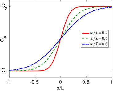
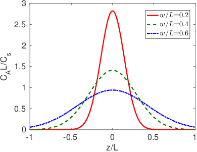
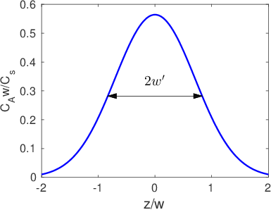
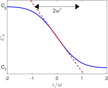
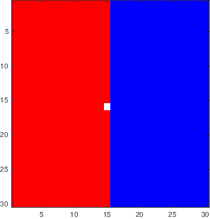
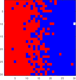
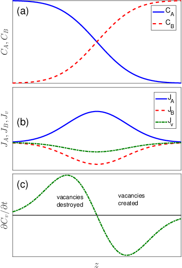
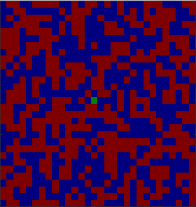


 Figure 5.5: The plane showing the function to be minimized and the circle showing the constraints, (from ref. [2]).


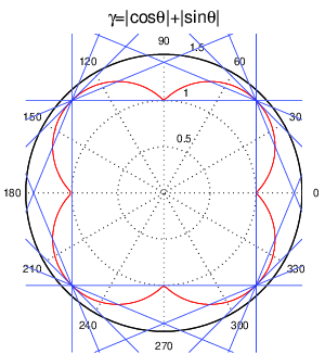
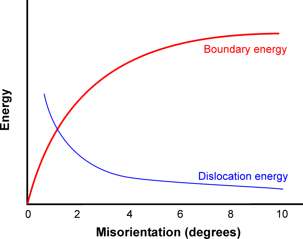 Figure 7.3: Grain boundary energy and energy per dislocation as a function of tilt angle according to the Read-Schockley model.

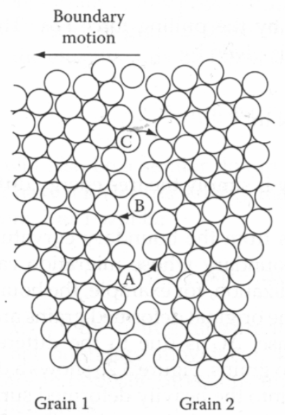
 Figure 7.9:


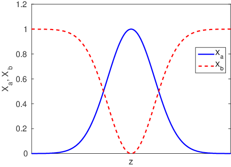


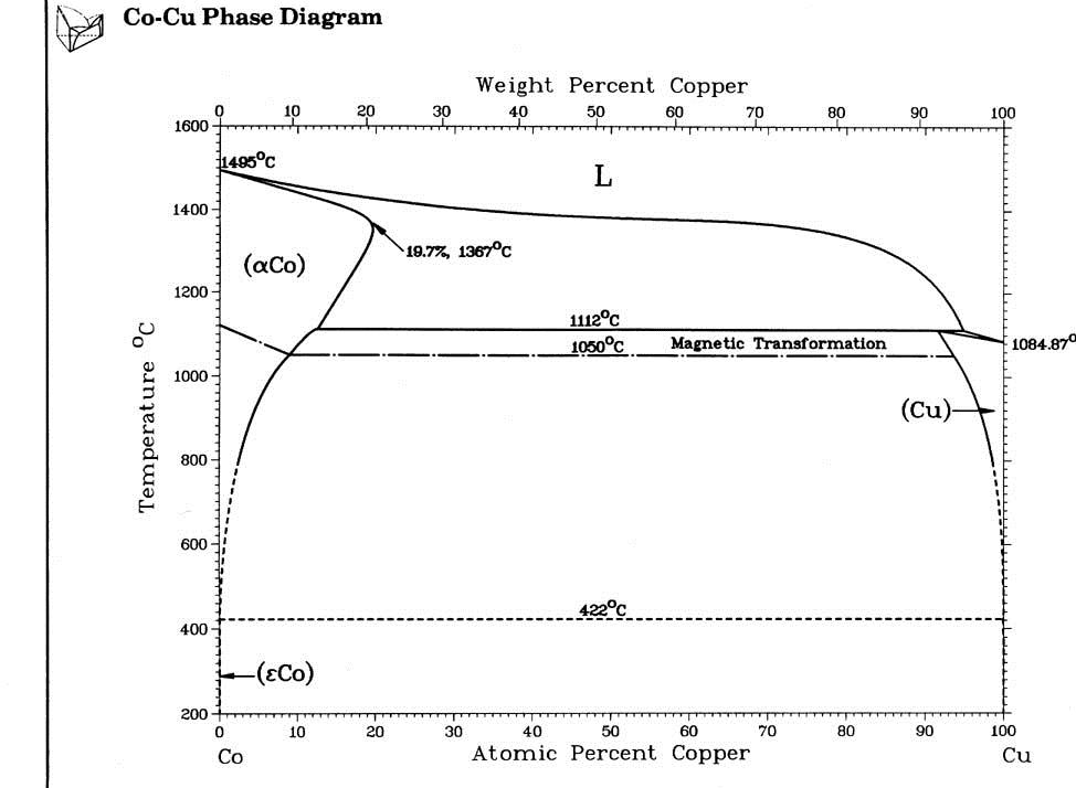
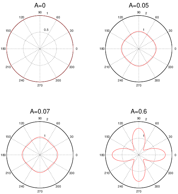
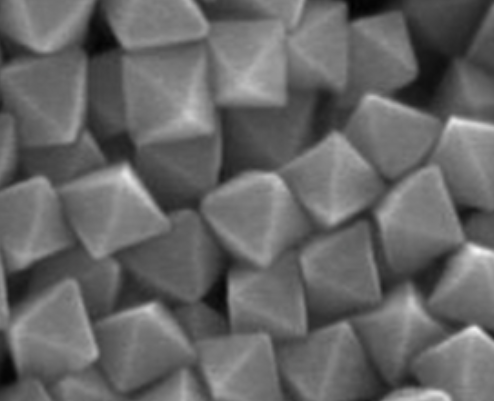


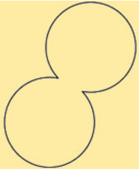
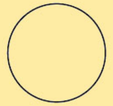
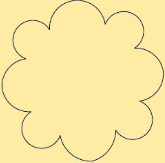
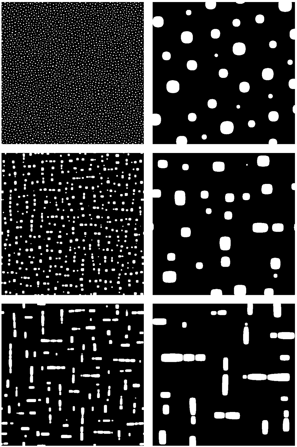


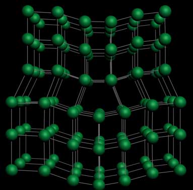


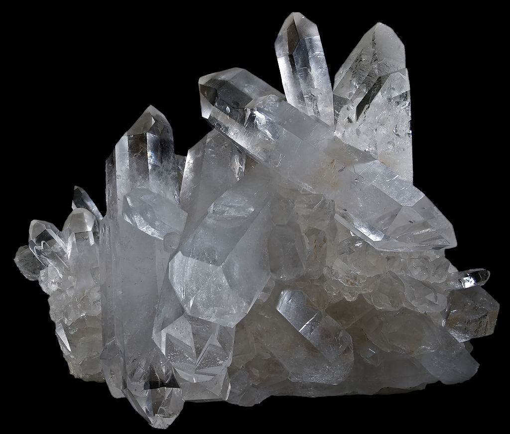
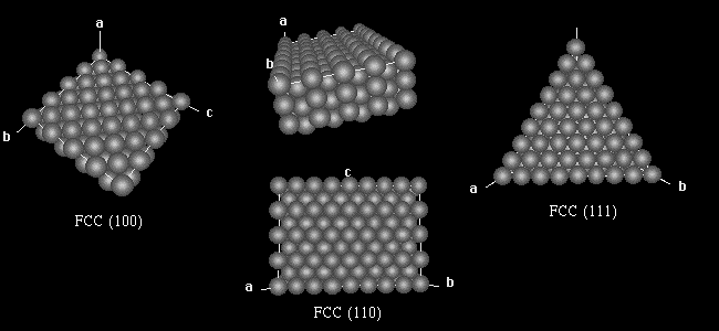


 e
e