316-2: Microstructural Dynamics II

Principles underlying development of microstructures. Defects, diffusion, phase transformations, nucleation and growth, thermal and mechanical treatment of materials. Lectures, laboratory. Prerequisite: 315 or equivalent.

2 Course Outcomes

At the conclusion of 316-2 students will be able to:

Predict nucleation rates from thermodynamic data
Describe where precipitates are likely to form in a multicomponent material
Design processing histories to obtain a desired microstructure
Correctly use and interpret TTT diagrams

3 Introduction

Much of this class is concerned with the appearance and growth of a new phase, referred to as

β

in Figure 3.1, from a matrix phase,

α .

In many cases the process can be divided into the following two phases:

A nucleation phase, where individual very small (typically in the nanometer range) $β$ precipitates are observed.
A growth phase where the $β$ precipitates grown in size.

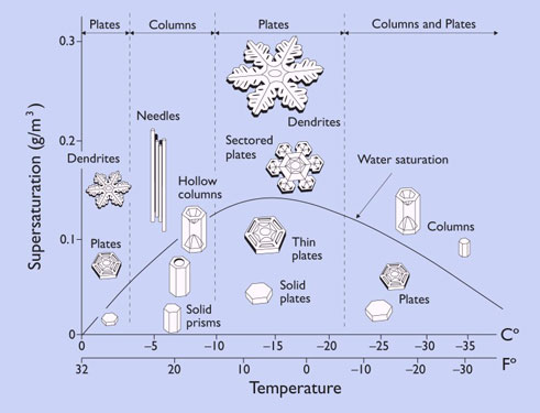
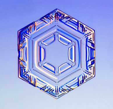
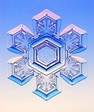
image: 4_home_ken_Mydocs_MSEcore_316-2_figures_drawing31.svg

Figure 3.1: Schematic Representation of Nucleation and Growth.

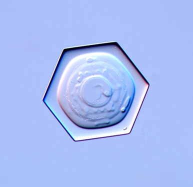
The process is actually much more interesting than one might think by looking at the simple example shown in Figure 3.1. Consider, for example, the images of snowflakes shown in figure 3.2.

image: 5_home_ken_Mydocs_MSEcore_316-2_figures_snowflake1.png

image: 6_home_ken_Mydocs_MSEcore_316-2_figures_snowflake2.png

image: 7_home_ken_Mydocs_MSEcore_316-2_figures_snowflake3.png

image: 8_home_ken_Mydocs_MSEcore_316-2_figures_snowflake4.png

image: 9_home_ken_Mydocs_MSEcore_316-2_figures_snowflake5.png

Figure 3.2: Snowflake images .

image: 10_home_ken_Mydocs_MSEcore_316-2_figures_snowmorphology.png

Figure 3.3: Morphology diagram for snowflakes .

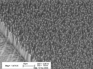
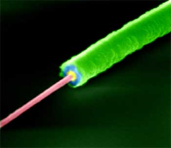
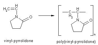
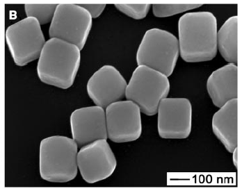
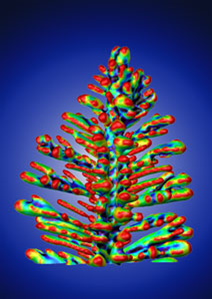
If you are not motivated by snowflakes, plenty of modern technological examples exist that illustrate the concepts developed in this course. Silicon nanowires illustrated below are one excellent example.

image: 11_home_ken_Mydocs_MSEcore_316-2_figures_nanowire_forest.png

image: 12_home_ken_Mydocs_MSEcore_316-2_figures_nanowire_falsecolor.png

Figure 3.4: Two examples of silicon nanowires .

image: 13_home_ken_Mydocs_MSEcore_316-2_figures_eutectic_alpha_ppt.svg

Figure 3.5: Generic eutectic phase diagram. A solid phase appears from the liquid as the temperature is cooled along the path indicated by the arrow.

The simplest example of these concepts is the freezing of pure water. The equilibrium phase at a given temperature is the one with the lowest molar free energy,

G_{m}

. A schematic representation of these free energies is shown in Figure 3.6. The free energies cross at 0

^{○}

C, with the liquid having a lower free energy at higher temperatures and the solid having a lower free energy at lower temperatures.

image: 14_home_ken_Mydocs_MSEcore_316-2_figures_liquid_and_solid_free_energy.svg

Figure 3.6: Schematic representation of the molar free energies of the solid and liquid phases of water.

Of course if we cool water below 0 °C, ice is not formed immediately - the solidification process takes time. Under appropriate conditions, it can be possible to maintain a liquid below its equilibrium melting point indefinitely, without ever seeing a solid. The ability to supercool a liquid is related to the fact that the interface between the solid and the liquid contributes a positive contribution to the overall free energy of the system.

Thermodynamics can be used to calculate the properties of equilibrium phases, including unstable equilibrium phases like the critical nucleus. The difference between a stable equilibrium (absolute minimum in free energy), a metastable equilibrium (local minimum in the free energy) and an unstable equilibrium (local maximum in the free energy) is illustrated in Figure 3.7.

image: 15_home_ken_Mydocs_MSEcore_316-2_figures_drawing1.svg

Figure 3.7: Energy as a function of nucleus size, illustrating stable, metastable and unstable states.

We need to compare the appropriate thermodynamic potentials for the cases where a critical nucleus is present and where it is absent. As illustrated schematically in Figure 3.8, we assume that the critical nucleus is spherical, with a radius of

R^{*}

image: 16_home_ken_Mydocs_MSEcore_316-2_figures_drawing32.svg

Figure 3.8: Initial and final states for the calculation of the work to form a critical nucleus.

Because of Laplace pressure, the pressure inside the critical nucleus is not equal to the pressure outside the critical nucleus. The correct thermodynamic potential to use is called the omega potential. The omega potential is relevant when a region of fixed volume is transformed from one phase to the other, in conditions where atoms are freely exchanged between the two phases. We consider this situation in more detail in the following section.

4 Homogeneous Nucleation in Unary Systems

Consider solidification of a pure compound from its melt as an example for a phase transformation L

\to β

in a unary system. Let's assume that the liquid phase L is homogeneous, i.e. there are no foreign objects or other surfaces in the system (such as container walls). We would like to understand the formation of a very small volume

V^{β^{*}}

of the solid phase, i.e. the nucleus, from the liquid. Note that we use

β^{*}

to indicate the nucleus (Figure 4). This is to remind ourselves that the composition of the nucleus is not necessarily identical to that of the final phase

β

at equilibrium (this is for the general case; in a unary system the composition cannot change). We will further assume that the nucleus shall be spherical with radius

R^{*}

image: 17_home_ken_Mydocs_MSEcore_316-2_figures_Lecture_02_Fig1.svg

Figure 4.1: Homogeneous nucleation in a unary system. Initially, the system only consists of the parent phase, here the liquid phase L. After nucleation, one infinitesimally small, spherical nucleus

β^{*}

is present also, surrounded by the parent phase L.

Before the formation of the nucleus, our system only contains L, at temperature

T^{L}

and pressure

P^{L}

. After, we also have to consider the temperature

T^{β^{*}}

and the pressure

P^{β^{*}}

of the nucleus.

The solidification shall be isothermal. Therefore,

\begin{matrix} T^{L} \equiv T^{β^{*}} & (4.1) \end{matrix}

What about the pressure? There is an interface between the nucleus and the liquid phase. The creation of this interface requires energy. As a consequence, the pressure in the nucleus is higher than in the liquid.

\begin{matrix} P^{β^{*}} > P^{L} & (4.2) \end{matrix}

As an analogy, consider inflating a rubber balloon against atmospheric pressure. Because of the energy stored in the stretched rubber membrane, the pressure on the inside of the balloon is higher than that on the outside.

We therefore need to determine the pressure differential

\begin{matrix} Δ P = P^{β^{*}} - P^{L} & (4.3) \end{matrix}

We will use the grand canonical (aka Landau, Omega) potential in the derivation of the free energy of the nucleus.

In our system, the grand canonical potential of the final state can be written as the sum

\begin{matrix} Ω = Ω_{b u l k}^{β^{*}} + Ω^{e x c} + Ω^{L}, & (4.4) \end{matrix}

where

Ω_{b u l k}^{β^{*}}

is contribution from the bulk of the nucleus,

Ω^{e x c}

is the surface excess free energy, i.e. the contribution from the interface, and

Ω^{L}

is the contribution from the liquid phase.

We can write the following:

\begin{matrix} Ω^{e x c} = γ_{L β^{*}} A_{L β^{*}}, & (4.5) \end{matrix}

where

γ_{L β^{*}}

is the interfacial free energy, with units

[γ] = \frac{J}{m^{2}}

, of the interface between the nucleus and the liquid phase, and

A_{L β^{*}}

is the interfacial area.

Recall that:

\begin{matrix} Ω = - P V & (4.6) \end{matrix}

We can therefore write Eq. 4.4 as

\begin{matrix} Ω = - P^{β^{*}} V^{β^{*}} - P^{L} V^{L} + γ_{L β^{*}} A_{L β^{*}} & (4.7) \end{matrix}

Generally speaking, we can see in Eq. 4.7 that the free energy of a small cluster (embryo) of the newly formed phase consists of negative terms that favor the formation, and positive terms that oppose the formation. The negative terms scale with the volume of the embryo, whereas the positive ones scale with the surface area. Therefore, if the surface-to-volume ratio is large, the embryo is unstable with respect to L. This means that it is much more likely to shrink than to grow. Conversely, if the surface-to-volume ratio is small, the embryo is stable with respect to L, and it is more likely to grow than to shrink. There is a critical size, at which the embryo is in unstable equilibrium, meaning that both shrinking and growing will reduce the free energy. This critical embryo is called the nucleus. In Figure 4.2, the free energy of an embryo of liquid water formed from water vapor is plotted against the radius. Note that this represents the condensation of a vapor rather than the solidification of a melt. Regardless, the thermodynamics are the same.

image: 18_home_ken_Mydocs_MSEcore_316-2_figures_Lecture_02_Fig2.svg

Figure 4.2: Free energy change as a function of the radius of an embryo of the new phase (here: spherical embryo of liquid water condensing from water vapor at a supercooling of 10 K). Free energy is released as the volume of the embryo increases. This component scales with

- R^{3}

(red line). However, energy is required to create the interface between the embryo and the parent phase. This term scales with

+ R^{2}

(green line). The latter term dominates at small

R

. Consequently, the sum of the two terms (blue line) goes through a maximum at the critical radius,

R^{*}

Because the nucleus is in unstable equilibrium,

\begin{matrix} {. \frac{d Ω}{d R} |}_{R^{*}} = 0 & (4.8) \end{matrix}

Performing this differentiation on Eq. 4.7,

\begin{matrix} - P^{β^{*}} {. \frac{d V^{β^{*}}}{d R} |}_{R^{*}} - P^{L} {. \frac{d V^{L}}{d R} |}_{R^{*}} + γ_{L β^{*}} {. \frac{d A_{L β^{*}}}{d R} |}_{R^{*}} + {. \frac{d γ_{L β^{*}}}{d R} |}_{R^{*}} A_{L β^{*}} = 0 & (4.9) \end{matrix}

We now make the very important assumption that the interfacial free energy

γ

does not change with the radius. In other words, that the interfacial free energy of the infinitesimally small nucleus is the same as that of a macroscopic interface. This assumption, known as the “capillarity assumption”, is convenient, and very likely wrong. How wrong, we do not know. So, with

{. \frac{d γ_{L β^{*}}}{d R} |}_{R^{*}} = 0

, we write

\begin{matrix} - P^{β^{*}} {. \frac{d V^{β^{*}}}{d R} |}_{R^{*}} - P^{L} {. \frac{d V^{L}}{d R} |}_{R^{*}} + γ_{L β^{*}} {. \frac{d A_{L β^{*}}}{d R} |}_{R^{*}} = 0 & (4.10) \end{matrix}

The total volume of our system is constant. Therefore, any increase in the volume of the nucleus must equal the decrease in volume of the liquid (Figure 4.10).

image: 19_home_ken_Mydocs_MSEcore_316-2_figures_Lecture_02_Fig3.svg

Figure 4.3: Volume conservation during nucleation. As the radius of the nucleus increases by

d R

, its volume increases by

\frac{d V}{d R}

. Because the total volume of the system is constant, the volume of the parent phase L shrinks by the same amount.

This allows us to rewrite Eq. 4.10,

\begin{matrix} - P^{β^{*}} {. \frac{d V^{β^{*}}}{d R} |}_{R^{*}} + P^{L} {. \frac{d V^{β^{*}}}{d R} |}_{R^{*}} + γ_{L β^{*}} {. \frac{d A_{L β^{*}}}{d R} |}_{R^{*}} & = 0 & (4.11) \\ \leftrightarrow - (P^{L} - P^{β^{*}}) {. \frac{d V^{β^{*}}}{d R} |}_{R^{*}} & = γ_{L β^{*}} {. \frac{d A_{L β^{*}}}{d R} |}_{R^{*}} & (4.12) \\ \leftrightarrow Δ P & = γ_{L β^{*}} \frac{{. \frac{d A_{L β^{*}}}{d R} |}_{R^{*}}}{{. \frac{d V^{β^{*}}}{d R} |}_{R^{*}}} & (4.13) \end{matrix}

Using the assumption that the nucleus is spherical, we can write

\begin{matrix} V^{β^{*}} (R) = \frac{4}{3} π R^{3} \Rightarrow {. \frac{d V^{β^{*}}}{d R} |}_{R^{*}} & = 4 π {R^{*}}^{2} & (4.14) \\ A_{L β^{*}} (R) = 4 π R^{2} \Rightarrow {. \frac{d A_{L β^{*}}}{d R} |}_{R^{*}} & = 8 π R^{*} & (4.15) \end{matrix}

With this,

\begin{matrix} Δ P = γ_{L β^{*}} \frac{8 π R^{*}}{4 π R^{2}} = \frac{2 γ_{L β^{*}}}{R^{*}} & (4.16) \end{matrix}

This pressure differential is called the Laplace pressure for the spherical nucleus (see also course notes for MSE 316-1). Note that for the derivation, we need not have assumed that the nucleus is spherical until solving Eqs. 4.15 and 4.15. For nuclei of different geometries, one could define a convenient critical length scale,

L^{*}

, instead. The Laplace pressure for such a nucleus would then follow from evaluating the differentials in Eqs. 4.15 and 4.15 at

L^{*}

Another way to evaluate the Laplace pressure for any interface is by considering the Laplace theorem

\begin{matrix} Δ P = γ (\frac{1}{R_{1}} + \frac{1}{R_{2}}) & (4.17) \end{matrix}

, where

R_{1}

and

R_{2}

are the principle radii of curvature.

Returning to the description of the nucleus, we can determine the reversible work of nucleation,

W_{r}^{*}

, as the difference between the free energy of the system at

R = R^{*}

and the free energy at

R = 0

, where the volume and area of the nucleus vanish.

\begin{matrix} W_{r}^{*} & = Ω (R = R^{*}) - Ω (R = 0) & (4.18) \\ = - P^{β^{*}} V^{β^{*}} + γ A - P^{L} V^{L} - (- P^{L} V_{0}^{L}), & (4.19) \end{matrix}

where

V_{0}^{L} = V^{L} + V^{β^{*}}

is the volume of L at before a nucleus forms, i.e. at

R = 0

. Plugging in, and collecting terms in two steps

\begin{matrix} W_{r}^{*} & = - P^{β^{*}} V^{β^{*}} + γ A - P^{L} (V^{L} - (V^{L} + V^{β^{*}})) & (4.20) \\ = - (P^{β^{*}} - P^{L}) V^{β^{*}} + γ A & (4.21) \\ = - Δ P V^{β^{*}} + γ A & (4.22) \end{matrix}

Assuming again that the nucleus is spherical,

\begin{matrix} W_{r}^{*} & = - Δ P (\frac{4}{3} π R^{* 3}) + γ (4 π R^{* 2}) & (4.23) \end{matrix}

Using Eq. 4.16, we write the critical radius

R^{*}

as a function of the Laplace pressure

\begin{matrix} R^{*} = \frac{2 γ}{Δ P} & (4.24) \end{matrix}

substitute into Eq. 4.23, and simplify

\begin{matrix} W_{r}^{*} & = - Δ P (\frac{4}{3} π {(\frac{2 γ}{Δ P})}^{3}) + γ (4 π {(\frac{2 γ}{Δ P})}^{2}) & (4.25) \\ = - \frac{32 π}{3} \frac{γ^{3}}{Δ P^{2}} + \frac{48 π}{3} \frac{γ^{3}}{Δ P^{2}} & (4.26) \\ \leftrightarrow W_{r}^{*} & = \frac{16 π}{3} \frac{γ^{3}}{Δ P^{2}} & (4.27) \end{matrix}

With this, we have determined the critical radius and reversible work of the spherical nucleus as a function of the Laplace pressure. It would be more convenient if we could replace this pressure, which is difficult to measure, by some other expression that we can evaluate. We will do this in the next section.

Recall that the nucleus is in unstable equilibrium with the parent phase, i.e. the phase that it formed from. At some temperature

T

, we can therefore write the following equality

\begin{matrix} G_{m}^{β^{*}} (T, P^{β^{*}}) = G_{m}^{L} (T, P^{L}) & (4.28) \end{matrix}

Let's consider a phase transformation that occurs as the temperature is lowered, such as a solidification from the melt. Let

Δ T = T_{m} - T

be the supercooling below the melting point

T_{m}

. We expect that the solidification is spontaneous if

Δ T > 0

. Recall also that

Δ P = P^{β^{*}} - P^{L}

The molar Gibbs free energies in Eq. 4.28 are energy surfaces of two variables. To simplify things, let's approximate

G_{m}

as a linear function in both

T

and

P

. We do this by writing the Taylor expansion of

G_{m}

and terminating it after the

1^{s t}

order terms. Because we know something about the equilibrium state, let's develop the Taylor expansion around the equilibrium point

(T_{m}, P^{L})

\begin{matrix} G_{m} (T, P) \approx G_{m} (T_{m}, P^{L}) + {. \frac{\partial G_{m}}{\partial T} |}_{T_{m}} \cdot (T - T_{m}) + {. \frac{\partial G_{m}}{\partial P} |}_{P^{L}} \cdot (P - P^{L}) & (4.29) \end{matrix}

Recall that

\begin{matrix} \frac{\partial G_{m}}{\partial T} & = - S_{m} & (4.30) \\ \frac{\partial G_{m}}{\partial P} & = V_{m} & (4.31) \end{matrix}

Let's now write the l.h.s. and r.h.s. of Eq 4.28 in terms of the Taylor expansion given in Eq. 4.29, and substitute the thermodynamic relationships given in Eqs. 4.31 and 4.31:

\begin{matrix} G_{m}^{β^{*}} (T, P^{β^{*}}) & = G_{m}^{β^{*}} (T_{m}, P^{L}) - S_{m}^{β^{*}} (T - T_{m}) + V_{m}^{β^{*}} (P^{β^{*}} - P^{L}) & (4.32) \\ G_{m}^{L} (T, P^{L}) & = G_{m}^{L} (T_{m}, P^{L}) - S_{m}^{L} (T - T_{m}) + V_{m}^{L} (P^{L} - P^{L}) & (4.33) \end{matrix}

Note that by using Eq. 4.31, we assume that the molar volume

V_{m}

is a constant, and does not change with changing pressure. This assumption of an incompressible nucleus is oftentimes reasonable in condensed matter, but can fail miserably when considering vapor phases.

Note that the third term on the r.h.s. of Eq. 4.33 vanishes. Further, because

(T_{m}, P^{L})

is the point of equilibrium, the first term on the r.h.s. of Eq. 4.33 is equal to the first term on the r.h.s. of Eq. 4.33. Finally, with the definitions for

Δ P

and

Δ T

, we rewrite Eq. 4.28 as:

\begin{matrix} S_{m}^{β^{*}} Δ T + V_{m}^{β^{*}} Δ P = S_{m}^{L} Δ T & (4.34) \\ \leftrightarrow & V_{m}^{β^{*}} Δ P = (S_{m}^{L} - S_{m}^{β^{*}}) Δ T & (4.35) \end{matrix}

Note that

\begin{matrix} S_{m}^{L} - S_{m}^{β^{*}} = Δ S_{m}^{○} & (4.36) \end{matrix}

where

Δ S_{f, m}^{○}

is the molar standard entropy of fusion (melting), i.e. the entropy gain associated with the opposite of the phase transformation that we are considering. This is simply the way the signs work out. When considering other phase transformations, for example melting, pay particular attention to getting the signs right in this step.

We substitute Eq. 4.36 into Eq. 4.35 and rearrange:

\begin{matrix} Δ P = \frac{Δ S_{m}^{○}}{V_{m}^{β^{*}}} Δ T & (4.37) \end{matrix}

Recall that at equilibrium,

\begin{matrix} Δ G_{m}^{○} (T_{m}) = 0 & (4.38) \\ \leftrightarrow & Δ H_{m}^{○} - T_{m} Δ S_{m}^{○} = 0 & (4.39) \\ \leftrightarrow & Δ S_{m}^{○} = \frac{Δ H_{m}^{○}}{T_{m}} & (4.40) \end{matrix}

This allows us to rewrite Eq. 4.37:

\begin{matrix} Δ P = \frac{Δ H_{f, m}^{○}}{V_{m}^{β^{*}} T_{m}} Δ T & (4.41) \end{matrix}

Equations 4.37 and 4.41 therefore allow us to estimate the Laplace pressure for any unary system for which we know the molar standard entropy of fusion, or the molar standard enthalpy of fusion and the melting temperature. These values are available for many pure phases. We can now express the critics radius and the reversible work of nucleation for a spherical, incompressible nucleus, using the capillarity approximation, as follows:

\begin{matrix} R^{*} & = \frac{2 γ}{Δ P} & (4.42) \\ = \frac{2 V_{m}^{β^{*}}}{Δ S_{m}^{○}} \frac{γ}{Δ T} & (4.43) \\ = \frac{2 V_{m}^{β^{*}} T_{m}}{Δ H_{f, m}^{○}} \frac{γ}{Δ T} & (4.44) \\ W_{r}^{*} & = \frac{16 π}{3} \frac{γ^{3}}{Δ P^{2}} & (4.45) \\ = \frac{16 π}{3} {(\frac{V_{m}^{β^{*}}}{Δ S_{f, m}^{○}})}^{2} \frac{γ^{3}}{Δ T^{2}} & (4.46) \\ = \frac{16 π}{3} {(\frac{V_{m}^{β^{*}} T_{m}}{Δ H_{f, m}^{○}})}^{2} \frac{γ^{3}}{Δ T^{2}} & (4.47) \end{matrix}

How do the Laplace pressure, critical radius, and the reversible work of nucleation depend on supercooling? Consider their graphs in Figure 4.4.

image: 20_home_ken_Mydocs_MSEcore_316-2_figures_Lecture_03_Fig1.svg

Figure 4.4: Scaling of the Laplace pressure

Δ P

, the critical radius

R^{*}

, and the reversible work of nucleation

W_{r}^{*}

, with supercooling

Δ T

. Graphs shown here correspond to the formation of a nucleus of liquid water from water vapor. A) Note the linear increase of the Laplace pressure with supercooling. At

Δ T = 0

, i.e.

T = T_{b}

Δ P = 0

. This means that the interface is flat (infinite radius of curvature). B) The critical radius is inversely proportional to

Δ T

. From this follows that small radii are expected at high supercooling, i.e. for temperatures far below the equilibrium temperature (here:

T_{b}

). At low supercooling, the critical radius increases quickly and approaches infinity as

Δ T \to 0

. An infinite radius is equivalent to a flat interface, but also means that nucleus is the size of the entire system. C) The reversible work is inversely proportional to

Δ T^{2}

and shows the same qualitative behavior as the critical nucleus. Because of the higher exponent, the effects are more pronounced. Close to the equilibrium temperature,

W_{r}^{*}

, which is an energetic barrier, becomes very large. Nucleation is therefore unlikely/very slow. The barrier quickly drops with increasing supercooling. In (D), the reversible work is expressed in units of

k T

As an example, consider the condensation of water vapor at

Δ T = 10 K

. In this case, the parent phase is the vapor phase (vap), and the nucleus is the liquid phase L. In Eq. 4.47 and Eq. 4.47, we further have to replace the entropy of fusion by the entropy of vaporisation. Keep in mind that we also replace the melting point by the boiling point.

\begin{matrix} R^{*} & = \frac{2 V_{m}^{L}}{Δ S_{v a p, m}^{○}} \frac{γ}{Δ T} & (4.48) \\ W_{r}^{*} & = \frac{16 π}{3} {(\frac{V_{m}^{L}}{Δ S_{v a p, m}^{○}})}^{2} \frac{γ^{3}}{Δ T^{2}} & (4.49) \end{matrix}

We find the following values in the literature:

γ = 72 \frac{m J}{m^{2}}

Δ S_{v a p, m}^{○} = 118.19 \frac{J}{m o l \cdot K}

T_{b} = 373.16 K

. The molar volume of the nucleus at the boiling point can be determined from the density of water at 372.16 K,

ρ_{3 73.16 K}^{H_{2} O} = 0.95805 \frac{g}{c m^{3}}

, and the molecular weight of water,

M_{w} = 18 \frac{g}{m o l}

. We find the molar volume as:

\begin{matrix} V_{m}^{L} = \frac{M_{w}}{ρ_{3 73.16 K}^{H_{2} O}} = \frac{18 \frac{g}{m o l}}{0.95805 \frac{g}{c m^{3}}} = \frac{18 \cdot 1 0^{- 6}}{0.95805} \frac{m^{3}}{m o l} \approx 1.879 \cdot 1 0^{- 5} \frac{m^{3}}{m o l} & (4.50) \end{matrix}

Plugging in,

\begin{matrix} R^{*} & = \frac{2 V_{m}^{L}}{Δ S_{v a p, m}^{○}} \frac{γ}{Δ T} & (4.51) \\ = \frac{2 \cdot 1.879 \cdot 1 0^{- 5} \frac{m^{3}}{m o l}}{118.19 \frac{J}{m o l \cdot K}} \frac{0.072 \frac{J}{m^{2}}}{10 K} & (4.52) \\ = 2.2891 \cdot 1 0^{- 9} m & (4.53) \\ \approx 2.3 n m & (4.54) \\ (4.55) \end{matrix}

\begin{matrix} W_{r}^{*} & = \frac{16 π}{3} {(\frac{V_{m}^{L}}{Δ S_{v a p, m}^{○}})}^{2} \frac{γ^{3}}{Δ T^{2}} & (4.56) \\ = \frac{16 π}{3} {(\frac{1.879 \cdot 1 0^{- 5} \frac{m^{3}}{m o l}}{118.19 \frac{J}{m o l \cdot K}})}^{2} \frac{{(0.072 \frac{J}{m^{2}})}^{3}}{{(10 K)}^{2}} & (4.57) \\ = 2.1954 \cdot 1 0^{- 17} J & (4.58) \\ \approx 2.20 \cdot 1 0^{- 17} J & (4.59) \end{matrix}

Let's also calculate the Laplace pressure for this case. Plugging into Eq. 4.37:

\begin{matrix} Δ P & = \frac{Δ S_{f, m}^{○}}{V_{m}^{β^{*}}} Δ T & (4.60) \\ = \frac{118.19 \frac{J}{m o l \cdot K}}{1.879 \cdot 1 0^{- 5} \frac{m^{3}}{m o l}} 10 K & (4.61) \\ = 6.2900 \cdot 1 0^{7} \frac{J}{m^{3}} & (4.62) \\ \approx 6.29 \cdot 1 0^{7} \frac{N m}{m^{3}} = 62.9 M P a & (4.63) \end{matrix}

Let's run a quick sanity check on the assumption that the nucleus is incompressible. The bulk modulus of water is

K = 2.15 G P a

. Using the definition of

K

and assuming linear bulk elasticity

\begin{matrix} K & = - \frac{d P}{d V} V_{0} & (4.64) \\ \Rightarrow K & = - \frac{Δ P}{Δ V} V_{0} & (4.65) \\ \leftrightarrow \frac{Δ V}{V_{0}} & = - \frac{Δ P}{K} & (4.66) \\ (4.67) \end{matrix}

Plugging in, we find the volumetric strain

\begin{matrix} \frac{Δ V}{V_{0}} & = - \frac{62.9 M P a}{2.15 G P a} & (4.68) \\ = - 0.0293 & (4.69) \\ \approx - 3 % & (4.70) \end{matrix}

Therefore, we would expect that assuming that the nucleus is incompressible, and ignoring the dependency of

V_{m}

on pressure will introduce only a small error into our calculation. Obviously, if the bulk modulus is higher, or the Laplace pressure lower, the error will have less of an impact.

5 Kinetics of Homogeneous Nucleation in Unary Systems

Microscopically, one of the assumptions of classical nucleation theory is that embryos of the new phase grow by addition of one monomer unit at a time, and shrink by dissociation of one monomer unit. In other words, embryos do not interact with each other. For an embryo with

n

monomer units, we can define forward and backward rates for these processes, as shown in Figure 1. At any given time

t

in our system, we can then count the number of embryos of size

n

and divide by the total volume to get the number density

ρ (n, t)

image: 21_home_ken_Mydocs_MSEcore_316-2_figures_Lecture_04_Fig1.svg

Figure 5.1: Embryos are assumed to grow by addition, and shrink by dissociation of one monomer unit. The monomer unit could be a metal atom, a water molecule, or a protein. This is reasonable as long as the density of embryos is so low that they do not encounter one another. For each embryo comprised of

n

monomer units, a forward (growth) rate

f (n)

and a backward (shrinkage) rate

b (n)

is defined.

The number of embryos of size

n

that are formed per unit time and volume, can the be expressed as

\begin{matrix} J (n) = ρ (n - 1) \cdot A (n - 1) \cdot β (n - 1) - ρ (n) \cdot A (n) \cdot α (n), & (5.1) \end{matrix}

where

A

is the surface area of the embryo,

β

is the total flux of monomers towards the embryo, and

α

is the evaporative flux, away from the embryo. These fluxes depend on the forward and backward rates.

Becker and Döring used this approach to determine the change in the number density of clusters over time and found that

\begin{matrix} \frac{\partial ρ (n, t)}{\partial (t)} = J (n) - J (n + 1) & (5.2) \end{matrix}

While a detailed analysis of this problem is beyond the scope of this class, a useful outcome is that for many systems relevant to us, it can be shown that a steady state is reached within

\sim 1 μ s

. Without going into detail, we will use the following formula for the steady state nucleation current

\begin{matrix} {\dot{N}}_{V} & = Z ν A_{n u c} ρ e^{- \frac{W_{r}^{*}}{k T}}, & (5.3) \\ [{\dot{N}}_{V}] & = \frac{1}{s \cdot c m^{3}} & (5.4) \end{matrix}

where

Z

is the dimensionless Zeldovich factor, i.e. the probability that a nucleus will become supercritical,

ν

is the impingement rate of monomers on the surface of the nucleus (

[ν] = \frac{1}{s \cdot c m^{2}}

A_{n u c}

is the surface area of the nucleus (

[A_{n u c}] = c m^{2}

), and

ρ

is the number density of monomers in the parent phase (

[ρ] = \frac{1}{c m^{3}}

). Because of the strong dependence of the reversible work of nucleation, and therefore the entire exponent, on temperature, we can frequently approximate the prefactor as a constant independent of temperature. In many unary (!!) condensed matter systems,

Z ν A_{n u c} \approx 1 0^{11} \frac{1}{s}

and

ρ \approx 1 0^{22} \frac{1}{c m^{3}} .

We can therefore use the following approximation in many cases:

\begin{matrix} {\dot{N}}_{V} \approx 1 0^{33} \frac{1}{s \cdot c m^{3}} e^{- \frac{W_{r}^{*}}{k T}} & (5.5) \end{matrix}

A technically useful nucleation current, i.e. a nucleation current that leads to a phase transformation in a “reasonable” amount of time, is

{\dot{N}}_{V} \geq 1 \frac{1}{s \cdot c m^{3}}

. Using eq. 5.5, what is the maximum value that the reversible work of nucleation can take?

\begin{matrix} {\dot{N}}_{V} \approx 1 0^{33} \frac{1}{s \cdot c m^{3}} e^{- \frac{W_{r}^{*}}{k T}} \geq 1 \frac{1}{s \cdot c m^{3}} & (5.6) \\ \leftrightarrow & e^{- \frac{W_{r}^{*}}{k T}} \geq 1 0^{- 33} & (5.7) \\ \leftrightarrow & \frac{W_{r}^{*}}{k T} {log}_{10} e \leq 33 & (5.8) \\ \leftrightarrow & \frac{W_{r}^{*}}{k T} \leq \frac{33}{{log}_{10} e} & (5.9) \\ \leftrightarrow & W_{r}^{*} ⪅ 76 k T & (5.10) \end{matrix}

This means that the barrier to nucleation, i.e. the reversible work, in a unary system, generally needs to be smaller or equal to

76 k T

(at the relevant temperature) in order to occur at a rate that is 'reasonable', i.e. of some technical use. We can use this value to quickly estimate whether we can expect to observe nucleation or not. Consider for example the condensation of water from its vapor for

Δ T ⪆ 20

K will

W_{r}^{*} < 76 k T .

Please note that this quick-and-dirty approach is only valid for unary systems.

It is instructive to consider the nucleation current

{\dot{N}}_{V}

as a function of

Δ T

. We can attempt to do so analytically, by considering all temperature-dependent variables in eq. 5.5, or numerically, e.g. using realistic values for all materials properties.For the analytical approach, write

{\dot{N}}_{V}

in a way that makes the temperature dependence more apparent:

\begin{matrix} {\dot{N}}_{V} & \approx 1 0^{33} \frac{1}{s \cdot c m^{3}} exp (- \frac{W_{r}^{*}}{k T}) & (5.11) \\ \Rightarrow {\dot{N}}_{V} & \propto exp (- \frac{c o n s t}{Δ T^{2} \cdot T}) & (5.12) \end{matrix}

Note that we have ignored small effects, such as the dependence of the molar volume (of a solid or liquid!) on temperature. Using the definition of

Δ T = T_{e q} - T

\begin{matrix} \Rightarrow {\dot{N}}_{V} & \propto exp (- \frac{c o n s t}{Δ T^{2} \cdot (T_{e q} - Δ T)}) & (5.13) \end{matrix}

We are interested in the interval from

Δ T = 0 (T = T_{e q})

T = 0 K (Δ T = T_{e q}

). By sketching out the terms in the denominator of the exponent, we can quickly get an idea of the overall shape of the graph of

{\dot{N}}_{V}

(Figure 5.2).

image: 22_home_ken_Mydocs_MSEcore_316-2_figures_Lecture_04_Fig2.svg

Figure 5.2: Sketching the graph of

{\dot{N}}_{V}

as a function of

Δ T

, Eq. 5.13. a) The denominator of the fraction in the exponent consists of two terms,

T_{e q} - Δ T

(green) and

Δ T^{2}

(blue). The denominator is the product of these terms (red). The product goes to zero at both side of the

Δ T

interval and has a maximum in between. Note that the each of the functions was sketched on a different

y

-axis. b) Next, we sketch the negative reciprocal of the product in (a). Note that the graph goes to negative infinity on either side of the

Δ T

interval and has a maximum at a negative value in between. c) Finally, we sketch Eq. 5.13, and find that

{\dot{N}}_{V}

goes to zero at either end of the interval, and goes through a maximum in between.

Using an appropriate graphing software, we can explore a specific example, for example the condensation of liquid water from vapor at ambient pressure (Figure 5.3).

image: 23_home_ken_Mydocs_MSEcore_316-2_figures_Lecture_04_Fig3.svg

Figure 5.3: Nucleation of liquid water from its vapor. Nucleation current

{\dot{N}}_{V}

is plotted on the

x

-axis, supercooling

Δ T

on the left

y

-axis, and the absolute temperature

T

on the right

y

-axis. Note that in b) and d) the very strong dependence of

{\dot{N}}_{V}

on temperature was made more apparent by plotting on a log scale. a) and b) show the entire physically relevant temperature range. c) and d) show the range in which

{\dot{N}}_{V}

passes through

1 s^{- 1} c m^{- 3}

. Note that

{\dot{N}}_{V} \to 0

for

Δ T \to 0

; this is because the reversible work of nucleation,

W_{r}^{*} \propto Δ T^{- 2}

, goes to infinity as

T \to T_{e q}

. Also,

{\dot{N}}_{V} \to 0

for

T \to 0

, because even a small barrier becomes insurmountable as the thermal energy of the system goes to zero. Finally, there is a pronounced maximum in

{\dot{N}}_{V}

, here at

Δ T \approx 250

K. At this temperature (

T \approx - 15 0^{○} C

), we would also have to consider direct nucleation of solid ice. This plot was created using Lecture_04_Fig3.m.

6 Heterogeneous Nucleation in Unary Systems

In this section, we will consider the impact of heterogeneity in the system. Specifically, we will assume the presence of a flat surface of some substrate

σ

. As before, we will look at the formation of a nucleus (phase:

β^{*}

) from a parent phase L. The major difference to the homogeneous case is that the shape of a nucleus formed at the interface between

σ

and L is generally not spherical. In addition, when determining the excess excess free energy of the nucleus, we will also have to consider interfacial free energies other than

γ_{L β^{*}}

. Let's first consider the shape of the nucleus.

image: 24_home_ken_Mydocs_MSEcore_316-2_figures_Lecture_05_Fig1.svg

Figure 6.1: Force balance at the triple line phase boundary for a small (axisymmetric) volume of the phase

β^{*}

at the interface between

σ

L. a) General case in which both horizontal and vertical forces are considered. b) Assuming an infinitely stiff substrate

σ

, vertical forces are ignored and

β^{*}

takes the shape of a spherical cap with contact angle

θ

Recall from MSE316-1, that the equilibrium shape at a triple line phase boundary (

L - σ - β^{*}

) results from the balance of the vector surface tension of the

L - σ

σ - β^{*}

, and

L - β^{*}

interfaces (Figure 1A). If we assume that

σ

is infinitely stiff, we can ignore the vertical force balance (Figure 1B). In the latter case,

β^{*}

takes the shape of a spherical cap with radius

R^{*}

and contact angle

θ

We find

θ

by considering the horizontal force balance only

\begin{matrix} γ_{L σ} & = γ_{σ β^{*}} + γ_{L β^{*}} cos θ & (6.1) \\ \leftrightarrow cos θ & = \frac{γ_{L σ} - γ_{σ β^{*}}}{γ_{L β^{*}}} & (6.2) \end{matrix}

image: 25_home_ken_Mydocs_MSEcore_316-2_figures_Lecture_05_Fig2.svg

Figure 6.2: 3D rendering of a nucleus of the phase

β^{*}

in the shape of a spherical cap, at the interface between substrate

σ

and the parent phase L.

To find the reversible work of heterogeneous nucleation, we consider the change in the grand canonical potential as we go from the initial to the final state

\begin{matrix} W_{r}^{*, h e t} & = Ω^{f} - Ω^{i} & (6.3) \\ = - Δ P V^{β^{*}} + γ_{L β^{*}} A_{L β^{*}} + γ_{σ β^{*}} A_{σ β^{*}} - γ_{L σ} A_{L σ}, & (6.4) \end{matrix}

where

V^{β^{*}}

is the volume of the nucleus,

A_{L β^{*}}

is the interfacial area between the nucleus and L, and

A_{σ β^{*}}

is the area of the interface between the substrate and the nucleus. While both these areas are created during nucleation, the area of the interface between the substrate and L,

A_{L σ}

, is removed in the process. Therefore, it enters into Eq. (3) as a negative term. Note that

A_{σ β^{*}} = A_{L σ}

(Figure 2).

By writing the volume and area terms in Eq. (3) as functions of

θ

, one can show that

\begin{matrix} W_{r}^{*, h e t} = W_{r}^{*} \cdot S (θ), & (6.5) \end{matrix}

where

W_{r}^{*}

is the reversible work of nucleation for the homogeneous case and the structure factor

S (θ)

is defined as

\begin{matrix} S (θ) = \frac{1}{4} (2 + cos θ) {(1 - cos θ)}^{2} & (6.6) \end{matrix}

Inspection of Eq. (6) and its graph (Fig. 3A,B) reveals the following properties

$θ \to 0^{○} \Rightarrow S (θ) \to 0$ , meaning that with decreasing contact angle (good wetting), the reversible work of nucleation is reduced substantially . For example, the structure factor is $1 0^{- 1}$ for $θ = 52. 5^{○}$ , $1 0^{- 2}$ for $θ = 28. 1^{○}$ , and $1 0^{- 3}$ for $θ = 15. 6^{○}$ (see Fig. 3C-E). Good wetting means that $cos θ \to 1$ , which, looking back at Eq. (2), requires that $γ_{L σ} > γ_{σ β^{*}}$ , i.e. that the free energy of the interface between nucleus and the substrate is lower than that between the liquid and the substrate.
$θ = 9 0^{○} \Rightarrow S (θ) = \frac{1}{2}$ , meaning that even for mediocre wetting, there is a substantial reduction in the barrier to nucleation (Fig. 3F). Mediocre wetting, where $cos θ \approx 0$ , occurs when $γ_{L σ} \approx γ_{σ β^{*}}$ .
$θ \to 18 0^{○} \Rightarrow S (θ) \to 1$ , meaning that for poor wetting the reversible work of heterogeneous nucleation approaches that of homogeneous nucleation. For example, the structure factor is $0.9$ for $θ = 127. 5^{○}$ and $0.99$ for $θ = 164. 5^{○}$ (Fig. 3 G,H). Poor wetting means that $cos θ \to - 1$ , which requires that $γ_{L σ} < γ_{σ β^{*}}$ .

image: 26_home_ken_Mydocs_MSEcore_316-2_figures_Lecture_05_Fig3_alt.svg

Figure 6.3: Plot of the structure factor for the spherical cap,

S (θ)

, vs. the contact angle

θ

using normal (a) and logarithmic (b) scaling of the

y

-axis.

Note that the critical radius

R^{*}

is the same in both homogeneous and heterogeneous nucleation and can be calculated as discussed earlier. However, the volume and surface area of the spherical cap are generally smaller.

\begin{matrix} R^{*, h e t} = R^{*, h o m} = R^{*} & (6.7) \end{matrix}

Using an approach similar to the one discussed in the homogeneous case, the heterogeneous nucleation current can be shown to be

\begin{matrix} {\dot{N}}_{V}^{h e t} = Z ν A_{n u c} ρ e^{- \frac{W_{r}^{*}}{k T} S (θ)} & (6.8) \end{matrix}

However, shape of the nucleus and the substrate impact the terms of the prefactor. We can frequently estimate

{\dot{N}}_{V}^{h e t}

in unary condensed matter systems as

\begin{matrix} {\dot{N}}_{V}^{h e t} \approx 1 0^{26} \frac{1}{s \cdot c m^{2}} \frac{A_{t o t}^{σ}}{V_{t o t}} e^{- \frac{W_{r}^{*}}{k T} S (θ)}, & (6.9) \end{matrix}

where

A_{t o t}^{σ}

is the total area of the nucleating surface, and

V_{t o t}

is the total volume of the system. In a simple case, this area could simply be the total area of the container walls, and the volume that of the container (and therefore, L before the transformation). However, nucleators could also be finely dispersed in the volume itself. Finally, in most real systems we would have to at least consider that there may be a distribution of nucleators of different potency (i.e. differing contact angle) on the container walls and dispersed in the bulk.

image: 27_home_ken_Mydocs_MSEcore_316-2_figures_Lecture_05_Fig4.svg

Figure 6.4: Heterogeneous nucleation in a v-shaped scratch. The angle enclosed by the sidewalls of the scratch and the

x y

plane is given by

α

. Note that the nucleus here takes the shape of a segment of a cylinder with radius

R^{*}

The structure factor also depends strongly on the assumptions we make regarding the shape of the substrate. For example, if we consider a nucleus forming in a v-shaped scratch in the surface (Fig. 4), we find that one can write the reversible work of nucleation as

\begin{matrix} W_{r}^{*, h e t} = W_{r}^{*} f (α, θ), & (6.10) \end{matrix}

where

α < 9 0^{○}

is the angle between the side walls and the horizontal plane, and

θ

is the contact angle. While

f (α, θ)

looks too intimidating to be shown here, its behavior is really very interesting:

\begin{matrix} α \to 0 & \Rightarrow f (α, θ) \to S (θ) & (6.11) \\ α > 0 & \Rightarrow f (α, θ) < S (θ) & (6.12) \\ θ - α \to + 0 & \Rightarrow f (α, θ) \to 0 & (6.13) \\ θ < α & \Rightarrow f (α, θ) = 0 & (6.14) \end{matrix}

This means that any scratch in a surface is a better nucleator than the smooth surface. Furthermore, if there are many scratches with a wide distribution of

α

in the substrate, and the contact angle

θ

is smaller than

9 0^{○}

, there will be at least a few for which the structure factor becomes vanishingly small. As a consequence, the reversible work of nucleation will become very small, and nucleation will occur quickly at these sites. As only one nucleus is in principle sufficient to initiate phase transformation (if growth is reasonably fast, which is not necessarily the case in solid state transformations), the most powerful nucleators can play an important role. It is therefore generally true that rough or porous substrates are more efficient nucleators.

However, if scratches or pores set in a smooth surface get very small, nuclei may not be able to grow out of them and into the bulk. Why? Hint: Consider the radius of curvature of the newly formed phase as it grows out of the scratch and compare it to the critical radius.

7 Nucleation in Binary Systems

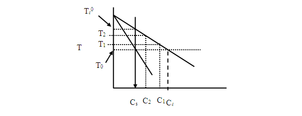
In the next couple of sections, we will take a look at nucleation in binary systems. Consider a typical precipitation in the solid state (Figure 1A). In this eutectic system with components 1 and 2, and the terminal solutions

α

(rich in component 2) and

β

(rich in component 1), we start with

α

at some initial mole fraction

X_{1}^{i}

and cool through the solvus line into the two-phase field, then hold at some temperature

T

. We are therefore considering the phase transformation

α \to α + β

. For now, let's pretend the system is homogeneous. From the phase diagram, we find the undercooling

Δ T = T_{e q} - T

(here, the relevant equilibrium temperature is given by the solvus line at

X_{1}^{i}

). Drawing the tie-line at

T

, we find the equilibrium mole fraction of component 1 in

α

X_{1, e q}^{α}

, and the equilibrium mole fraction of component 1 in

β

X_{1, e q}^{β}

. The supersaturation of undercooled

α

T

Δ X = X_{1}^{i} - X_{1, e q}^{α}

Next, let's first look at the driving force for phase transformation. For this, consider the

G X

diagram corresponding to temperature

T

that underlies the

T X

(phase) diagram (Figure 1B). The free energy of the

α

phase as a function of the mole fraction of component 1 at temperature

T

and pressure

P^{α}

is given by

G_{m}^{α} (T, P^{α}, X_{1})

, that of

β

G_{m}^{β} (T, P^{α}, X_{1})

. The initial state of the system is that of a homogenous, but supersaturated/undercooled

α

with

G_{m}^{α} (T, P^{α}, X_{1}^{i})

(point I). To reduce the free energy,

β

precipitates enriched in component 1 form from the matrix

α

, depleting the matrix of component 1 in the process. Equilibrium is reached where

X_{1} = X_{1}^{i}

intersects the common tangent (point F). In this state, the mole fraction of component 1 in

α

is that of the point of tangency,

X_{1, e q}^{α}

, and that in

β

X_{1, e q}^{β}

. The free energy of the system in this state can be calculated by calculating the weighted sum

X_{α} G_{m}^{α} (T, P^{α}, X_{1, e q}^{α}) + X_{β} G_{m}^{β} (T, P^{α}, X_{1, e q}^{β})

, using the lever rule to determine

X_{α}

and

X_{β}

. The change in free energy associated with the phase transformation,

Δ G_{m}^{α \to α + β}

, is identical to the negative distance

\bar{F I}

. Note, however, that we consider here both phases at the same pressure

P^{α}

. This means that the Laplace pressure and the curvature of the interface is zero. This corresponds to complete phase separation as shown in Figure 1C.

image: 28_home_ken_Mydocs_MSEcore_316-2_figures_Lecture_06_07_Fig1.svg

Figure 7.1: Phase transformation in a binary system. a) Generic binary eutectic phase

(T X)

diagram. b)

G X

diagram for the system at temperature

T

in (a). The free energy change

Δ G_{m}^{α \to α + β}

corresponds to the energy per mole of

α

converted, i.e. the overall driving force. c) Schematic drawing that corresponds to the initial and final equilibrium states referenced in (a) and (b). Note that the

α - β

interface has no curvature, therefore

Δ P = 0

Instead of looking at the free energy change for the overall phase transformation, we need to consider the free energy change associated with the formation of the nucleus from the parent phase (Figure 2). Let's assume the nucleus is spherical with radius

R^{*}

and incompressible.

image: 29_home_ken_Mydocs_MSEcore_316-2_figures_Lecture_06_07_Fig2.svg

Figure 7.2: Schematic drawing showing the initial state of the homogeneous

α

(T, P^{α}, X_{1}^{i})

, and the unstable equilibrium of one very small, spherical nucleus

β^{*}

with radius

R^{*}

(T, P^{β^{*}}, X_{1}^{'})

with the surrounding matrix

α

. Note that the transformation is isothermal and the nucleus so small that its formation does not change the composition of

α

Recall that if we assume incompressibility,

\begin{matrix} \frac{\partial G_{m}}{\partial P} = V_{m} & (7.1) \\ \Rightarrow & \frac{Δ G_{m}}{Δ P} = V_{m} & (7.2) \\ \leftrightarrow & \frac{G_{m} (T, P^{f}, X_{1}) - G_{m} (T, P^{i}, X_{1})}{(P^{f} - P^{i})} = V_{m} & (7.3) \\ \leftrightarrow & G_{m} (T, P^{f}, X_{1}) = G_{m} (T, P^{i}, X_{1}) + V_{m} Δ P & (7.4) \end{matrix}

This means in the

G X

diagram, increasing the pressure from an initial value

P^{i}

to a final value

P^{f}

for any given phase simply shifts the free energy to higher energy by the amount

V_{m} Δ P

, where

Δ P = P^{f} - P^{i}

For the nucleus, this means that

\begin{matrix} G_{m}^{β} (T, P^{β^{*}}, X_{1}) = G_{m}^{β} (T, P^{α}, X_{1}) + V_{m}^{β} Δ P & (7.5) \end{matrix}

V_{m}^{β} Δ P \geq 0

is therefore the contribution of the interface to the molar free energy of the nucleus. In unstable equilibrium, this must be exactly balanced by the free energy released when a solid of the composition of the nucleus is formed from the matrix. One way to think about this scenario is to consider the corresponding

G X

diagram (Fig. 3).

The major difference between Fig. 3 and Fig. 1B is that we now also consider the unstable equilibrium of the matrix at composition

X_{1}^{i}

with the nucleus. We know that there must be a common tangent between the free energy curves for the matrix and the nucleus. One of the points of tangency is

G_{m}^{α} (P^{α}, X_{1}^{i})

and the slope of the tangent is equal to the slope of

G_{m}^{α}

X_{1}^{i}

. A priori, we do not know what value

P^{β^{*}}

takes, but really all we need to do is shift

G_{m}^{β} (P^{α}, X_{1})

vertically until there is a point of tangency to the tangent in

G_{m}^{α}

. The vertical shift is then exactly equal to

V_{m}^{β} Δ P

and the point of tangency indicates the composition of the nucleus,

X_{1}^{'}

image: 30_home_ken_Mydocs_MSEcore_316-2_figures_Lecture_06_07_Fig3.svg

Figure 7.3: Schematic

G X

diagram for a binary system at temperature

T

α

is given for

P^{α}

(purple line). For

β

, molar free energies at

P^{α}

(green dashed line) and

P^{β^{*}}

(green line) are given; the latter is shifted to higher free energy by

V_{m}^{β} Δ P

. The first of two common tangents is for the final equilibrium between matrix

α

at composition

X_{1, e q}^{α}

and pressure

P^{α}

, and precipitate

β

at composition

X_{1, e q}^{β}

and pressure

P^{α}

(cyan dashed line), similar to the common tangent in Figure 1B. The second is for the unstable equilibrium between the matrix

α

with composition

X_{1}^{i}

and pressure

P^{α}

, and nucleus with composition

X_{1}^{'}

and pressure

P^{β^{*}}

(red dashed line).

By inspection, we find that

\begin{matrix} G_{m}^{β} (P^{α}, X_{1}^{'}) + V_{m} Δ P - G_{m}^{α} (P^{α}, X_{1}^{i}) = {. \frac{\partial G_{m}^{α}}{\partial X_{1}} |}_{X_{1}^{i}} (X_{1}^{'} - X_{1}^{i}) & (7.6) \\ \leftrightarrow & - V_{m} Δ P = G_{m}^{β} (P^{α}, X_{1}^{'}) - G_{m}^{α} (P^{α}, X_{1}^{i}) - {. \frac{\partial G_{m}^{α}}{\partial X_{1}} |}_{X_{1}^{i}} (X_{1}^{'} - X_{1}^{i}) & (7.7) \end{matrix}

Now let's see whether we can show that the r.h.s. of Eq. (7.7) is indeed the molar free energy change for the formation of a nucleus, i.e. the Gibbs free energy change associated with the formation of an infinitesimal amount of material with a composition

X_{1}^{'}

that is different from the initial composition

X_{1}^{i}

. This amount shall be so small that the mole fractions of the componenta 1 and 2 in the matrix shall not change. We can then calculate the Gibbs free energy change by

removing a small amount of material of composition $X_{1}^{'}$ from a large amount of material of composition $X_{1}^{i}$ .
forming the same small amount of material of composition $X_{1}^{'}$ .

Note that the free energy required to remove material is not equal to the free energy gained because the system is closed and the total number of atoms is fixed.

Step 1. The free energies of the initial and final states of the matrix

α

are then

\begin{matrix} G^{α, i} & = G^{α} (n_{1}^{i}, n_{2}^{i}) & (7.8) \\ G^{α, f} & = G^{α} (n_{1}^{f}, n_{2}^{f}) & (7.9) \end{matrix}

, where the number of atoms of component

j

in the initial state is given by

n_{j}^{i}

and that in the final state given by

n_{j}^{f}

For a very small number of atoms

n_{j}^{'} = n_{j}^{f} - n_{j}^{i}

removed, we can expand

G^{α, f}

around

G^{α, i}

to first order only. At constant

T

and

P^{α}

Using the definition of the chemical potential

μ_{j} = \frac{\partial G}{\partial n_{j}}

, the free energy change can be written as

\begin{matrix} Δ G^{r} & = G^{α, f} - G^{α, i} & (7.10) \\ = μ_{1}^{α} (X_{1}^{i}) (n_{1}^{f} - n_{1}^{i}) + μ_{2}^{α} (X_{1}^{i}) (n_{2}^{f} - n_{2}^{i}) & (7.11) \\ = - μ_{1}^{α} (X_{1}^{i}) n_{1}^{'} - μ_{2}^{α} (X_{1}^{i}) n_{2}^{'} & (7.12) \end{matrix}

To find the molar free energy change associated with the removal from the matrix, we divide by the total number of moles of removed,

n_{t o t}^{'} = n_{1}^{'} + n_{2}^{'}

\begin{matrix} Δ G_{m}^{r} = - μ_{1}^{α} (X_{1}^{i}) X_{1}^{'} - μ_{2}^{α} (X_{1}^{i}) X_{2}^{'} & (7.13) \end{matrix}

Step 2. The free energy of formation for an infinitesimal amount of material of composition

X_{1}^{'}

is simply its molar free energy.

\begin{matrix} G_{m}^{β} (X_{1}^{'}) = μ_{1}^{β} (X_{1}^{'}) X_{1}^{'} + μ_{2}^{β} (X_{1}^{'}) X_{2}^{'} & (7.14) \end{matrix}

Step 3. The total free energy change for removal and formation of material of composition

X_{1}^{'}

from a matrix of composition

X_{1}^{i}

is then the sum of Eq. (7.13) and Eq. (7.14).

\begin{matrix} Δ G_{m}^{α \to β^{*}} & = Δ G_{m}^{r} + G_{m}^{β} (X_{1}^{'}) & (7.15) \\ = [μ_{1}^{β} (X_{1}^{'}) - μ_{1}^{α} (X_{1}^{i})] X_{1}^{'} + [μ_{2}^{β} (X_{1}^{'}) - μ_{2}^{α} (X_{1}^{i})] X_{2}^{'} & (7.16) \end{matrix}

This is a very general result that can be used even if the difference in mole fractions is large, as long as only a small amount of

β^{*}

is made.

But for our purposes, we just substitute Eq. (7.13) in Eq. (7.16)

\begin{matrix} Δ G_{m}^{α \to β^{*}} = G_{m}^{β} (X_{1}^{'}) - μ_{1}^{α} (X_{1}^{i}) X_{1}^{'} - μ_{2}^{α} (X_{1}^{i}) X_{2}^{'} & (7.17) \end{matrix}

Separately, we express

G_{m}^{α} (X_{1}^{i})

in terms of the chemical potentials, rearrange to

\begin{matrix} 0 = - G_{m}^{α} (X_{1}^{i}) + μ_{1}^{α} (X_{1}^{i}) X_{1}^{i} + μ_{2}^{α} (X_{1}^{i}) X_{2}^{i} & (7.18) \end{matrix}

, and then add the l.h.s. of Eq. (7.17) to the l.h.s of Eq. (7.18) and the r.h.s. of Eq. (7.17) to the r.h.s of Eq. (7.18)

\begin{matrix} Δ G_{m}^{α \to β^{*}} = G_{m}^{β} (X_{1}^{'}) - G_{m}^{α} (X_{1}^{i}) + μ_{1}^{α} (X_{1}^{i}) (X_{1}^{i} - X_{1}^{'}) + μ_{2}^{α} (X_{1}^{i}) (X_{2}^{i} - X_{2}^{'}) & (7.19) \end{matrix}

Substituting

X_{2} = 1 - X_{1}

\begin{matrix} Δ G_{m}^{α \to β^{*}} = G_{m}^{β} (X_{1}^{'}) - G_{m}^{α} (X_{1}^{i}) + [μ_{1}^{α} (X_{1}^{i}) - μ_{2}^{α} (X_{1}^{i})] (X_{1}^{i} - X_{1}^{'}) & (7.20) \end{matrix}

Finally, with we can express the change in free energy in terms of the Gibbs free energies

As we fixed the pressure at

P^{α}

, this is identical to

Finally, comparison of Eq. (0.1) and Eq. (7.7) reveals that the right hand sides are identical. This means that the left hand side must also be identical

One can further show that for small

Δ X = X_{1}^{i} - X_{1, e q}^{α}

Using the definition of the supersaturation and substituting into Eq. (0.1) , where C is (nearly) constant

With this, we can calculate the critical radius for the spherical, incompressible nucleus, and the reversible work of nucleation for the binary case.

\begin{matrix} R^{*} & = \frac{2 V_{m}}{C} \frac{γ}{Δ X} & (7.21) \\ W_{r}^{*} & = \frac{16 π}{3} {(\frac{V_{m}}{C})}^{2} \frac{γ^{3}}{Δ X^{2}} & (7.22) \end{matrix}

These expressions resemble those we found for unary systems. Note how the supersaturation

Δ X

replaces the undercooling

Δ T

, and

C

takes the places of

Δ S_{m}^{○}

. Because

Δ T

and

Δ X

are not independent variables, they can be used interchangeably when discussing effects qualitatively.

8 Strain Effects in Nucleation

Some of the most interesting phase transformations in materials science occur in the solid state. In this case, we need to consider the effect of strain at the interface between the nucleus and the matrix. Recall that strain is unique to solid-solid, coherent or semi-coherent interfaces. Strain is caused by lattice mismatch across the interface and results in an elastic deformation of bonds. We can define an elastic strain energy density,

W_{V}^{e l}

, that is equal to the total strain energy divided by the volume of the nucleus

\begin{matrix} W_{V}^{e l} = \frac{W_{t o t}^{e l}}{V^{β}} [W_{V}^{e l}] = \frac{J}{m^{3}} = P a & (8.1) \end{matrix}

We can therefore write down the grand canonical potential of the system

\begin{matrix} Ω = - P^{β} V^{β} - P^{α} V^{α} + γ_{α β} A^{α β} + W_{V}^{e l} V^{β} & (8.2) \end{matrix}

In unstable equilibrium, for a spherical nucleus with critical radius

R^{*}

Using

, and collecting terms

For the spherical nucleus, we substitute volume and area, differentiate, and rearrange

\begin{matrix} R^{*} = \frac{2 γ_{α β}}{Δ P - W_{V}^{e l}} & (8.3) \end{matrix}

It is equally straightforward to show that

\begin{matrix} W_{r}^{*} = \frac{16 π}{3} \frac{γ_{α β}^{3}}{{(Δ P - W_{V}^{e l})}^{2}} & (8.4) \end{matrix}

Therefore, both

R^{*}

and

W_{r}^{*}

increase with increasing

W_{V}^{e l}

. In other words, strain makes it more difficult for nucleation to occur. Note that for

W_{V}^{e l} \to Δ P

R^{*} \to \infty

and

W_{r}^{*} \to \infty

Δ T

(unary case) or

Δ X

(binary case) approach zero, i.e. when the state of the system approaches the solvus line. Strain can therefore be thought as shifting the solvus to lower temperature. For the unary case We introduce the effective undercooling/supersaturation

\begin{matrix} u n a r y & Δ P - W_{V}^{e l} = C_{u} Δ T^{e f f} & (8.5) \\ \leftrightarrow & C_{u} Δ T - W_{V}^{e l} = C_{u} Δ T^{e f f} & (8.6) \\ \leftrightarrow & Δ T^{e f f} = Δ T - \frac{W_{V}^{e l}}{C_{u}} & (8.7) \\ b i n a r y & Δ P - W_{V}^{e l} = C_{b} Δ X^{e f f} & (8.8) \\ \leftrightarrow & Δ X^{e f f} = Δ X - \frac{W_{V}^{e l}}{C_{b}} & (8.9) \end{matrix}

This allows us to define define the shift of the equilibrium temperature in the unary case, and of the solvus line in the binary case (Figure 1).

\begin{matrix} u n a r y Δ Δ T = \frac{W_{V}^{e l}}{C_{u}} & b i n a r y & Δ Δ X = \frac{W_{V}^{e l}}{C_{b}} & (8.10) \end{matrix}

image: 31_home_ken_Mydocs_MSEcore_316-2_figures_Lecture_08_09_Fig1.svg

Figure 8.1: Effect of strain on the solvus in a binary system. a) Schematic

G X

diagram. Elastic strain energy shifts

G_{m}^{β}

to higher energy. Note that this shift is addition to the shift

Δ P V_{m}

that results from any curvature of the interface. As a consequence, a new equilibrium is established and the equilibrium compositions shift to new values,

X_{1, e q}^{α, s t r}

and

X_{1, e q}^{β, s t r}

. b) In the phase diagram, the shift of the equilibrium in the presence of strain is equivalent to a shift of the solvus by

Δ Δ X = X_{1, e q}^{α, s t r} - X_{1, e q}^{α}

. As a consequence the effective supersaturation is reduced.

One could conclude that the reversible work of nucleation for coherent, strained nuclei should always be larger than that for incoherent nuclei, where there is no strain. However, the interfacial free energy of the coherent interface,

γ_{C}

, can be considerably smaller than that of the totally incoherent interface,

γ_{i} .

We therefore have to compare

\begin{matrix} W_{r}^{*, c} & = \frac{16 π}{3} \frac{γ_{C}^{3}}{{(C_{b} Δ X - W_{V}^{e l})}^{2}} & (8.11) \\ W_{r}^{*, i} & = \frac{16 π}{3} \frac{γ_{i}^{3}}{{(C_{b} Δ X)}^{2}} & (8.12) \end{matrix}

Comparing the graphs of Eq. (8.12) and Eq. (8.12), it is apparent that the asymptote of

W_{r}^{*, c}

is shifted by

Δ Δ X = \frac{W_{V}^{e l}}{C_{b}}

towards greater

Δ X

(Figure 2). For small

Δ X

, therefore

W_{r}^{*, i} < W_{r}^{*, c}

, and we expect incoherent nuclei to form faster. However, as

Δ X

is small, the nucleation current will be small. For large

Δ X

, we can neglect the contribution of the strain energy density to the denominator in Eq. (8.12). With

γ_{i} > γ_{C}

, we find that the barrier

W_{r}^{*, i} > W_{r}^{*, c}

; therefore coherent nuclei form more readily.

image: 32_home_ken_Mydocs_MSEcore_316-2_figures_Lecture_08_09_Fig2.svg

Figure 8.2: Plot of the reversible work of nucleation for incoherent (blue line) and coherent nuclei (red line), using

γ_{i} = 0.5 {J m}^{- 2}

;

γ_{C} = 0.2 {J m}^{- 2}

;

W_{V}^{e l} = 2 G P a

;

C_{b} = 50 G P a

Q: Derive an expression for the supersaturation at which there is a crossover between

W_{r}^{*, c}

and

W_{r}^{*, i}

. Discuss the dependence of

Δ X_{x o}

on the ratio of the interfacial free energies and other relevant properties.

Q: Replot Figure 2 with the

W_{r}^{*}

expressed in units of

k T

. Assume that the solvus temperature at

Δ X = 0

is 473 K, and that the solvus is linear with a slope of 100 K. Discuss the expected nucleation rate for coherent and incoherent nuclei as a function of

Δ X

If we assume that the nucleus is not only spherical and incompressible, and that the capillarity assumption holds, but also that the interface between nucleus

(β)

and matrix

(α)

is coherent and that both are elastically isotropic, the elastic strain energy density has a simple form

\begin{matrix} W_{V}^{e l} = 18 ε^{2} \frac{μ^{α} K^{β}}{3 K^{β} + 4 μ^{α}}, & (8.13) \end{matrix}

where

K^{β}

is the bulk modulus of the nucleus,

μ^{α}

is the shear modulus of the matrix, and

ε

is the misfit parameter.

We can then consider two limiting cases,

a soft nucleus in a stiff matrix, $μ^{α} ≫ K^{β}$ $\begin{matrix} W_{V}^{e l} \approx 18 ε^{2} \frac{μ^{α} K^{β}}{3 K^{β} + 4 μ^{α}} = \frac{9}{2} ε^{2} \frac{μ^{α} K^{β}}{μ^{α}} = \frac{9}{2} ε^{2} K^{β} & (8.14) \end{matrix}$
a stiff nucleus in a soft matrix, $K^{β} ≫ μ^{α}$ $\begin{matrix} W_{V}^{e l} \approx 18 ε^{2} \frac{μ^{α} K^{β}}{3 K^{β} + 4 μ^{α}} = 6 ε^{2} \frac{μ^{α} K^{β}}{K^{β}} = 6 ε^{2} μ^{α} & (8.15) \end{matrix}$

Finally, if we assume that matrix and nucleus both have cubic structure

\begin{matrix} ε & = \frac{1}{3} \frac{V_{m}^{β} - V_{m}^{α}}{V_{m}^{α}} & (8.16) \\ ε & \approx \frac{a^{β} - a^{α}}{a^{α}}, & (8.17) \end{matrix}

where

V_{m}

is the molar volume and

a

the lattice parameter.

9 Kinetics of Nucleation in the Solid State

The nucleation current for homogeneous nucleation in unary systems can be written in the form of an Arrhenius law with several prefactors that, to first order, we can approximate by a constant.

\begin{matrix} {\dot{N}}_{V} = Z ν A_{n u c} ρ e^{- \frac{W_{r}^{*}}{k T}} \approx 1 0^{33} \frac{1}{s \cdot c m^{3}} e^{- \frac{W_{r}^{*}}{k T}} & (9.1) \end{matrix}

Recall that

ρ

is the number density of monomer units and the product

Z ν A_{n u c}

can be interpreted as the frequency at which monomer units attach successfully to the nucleus. In unary systems, we can get away with ignoring the temperature dependence of this frequency. However, in binary and multicomponent systems, where thermally activated diffusion becomes much more important, we write instead

\begin{matrix} {\dot{N}}_{V} = ω e^{- \frac{Δ G_{d}}{k T}} ρ e^{- \frac{W_{r}^{*}}{k T}} = ω ρ e^{- \frac{Δ G_{d} + W_{r}^{*}}{k T}}, & (9.2) \end{matrix}

where

ω

is again an attachment frequency with units of [s

^{- 1}

], and

Δ G_{d}

is the free energy of activation for the relevant diffusive processes. We can directly see that all other things remaining equal, the nucleation rate decreases if

Δ G_{d}

increases. We therefore expect nucleation to be more rapid where diffusion is “easy”.

Previously, we found that the nucleation rate in unary systems increases with increasing supercooling, because the reversible work of nucleation decreases (

W_{r}^{*} \propto Δ T^{- 2}

), but eventually decreases again at very low temperatures because it becomes impossible for the system to overcome even a small (but finite) barrier (section 4, Figures 2 and 3). In binary systems, the reversible work of nucleation instead is proportional to

Δ X^{- 2}

(section XYZ).

Δ T

is of course a function of

Δ X

, and for the sake of the following discussion let's pretend this function is linear. This is equivalent of assuming that the solvus is a straight line. If so, then we only need to consider the impact of the additional exponential term in binary systems (Figure 1). The term

e^{- \frac{Δ G_{d}}{k T}}

goes to unity at high temperatures and decreases rapidly as the temperature decreases. Generally speaking, this reduces the nucleation rate across the board, but especially so at low temperatures. It also shifts the maximum rate to slightly higher temperature, i.e. lower supercooling.

image: 33_home_ken_Mydocs_MSEcore_316-2_figures_Lecture_10_11_Fig1.svg

Figure 9.1: Dependence of the nucleation current

{\dot{N}}_{V}

(black line) on temperature

T

{\dot{N}}_{V}

is proportional to the product of two exponential terms. One is dependent on the reversible work of nucleation (blue dashed line), which itself is dependent on temperature, and approaches zero for temperatures approaching the equilibrium temperature (where the barrier is infinite) and absolute zero (where the thermal energy is insufficient to overcome even a small, but finite barrier). This term goes through a maximum between at an intermediate temperature. The other term represents diffusive processes (red dashed line), which increase with increasing temperature but are strongly attenuated at low temperature. The product of the two terms, and therefore the nucleation current, has the same general shape as the first term. However, the maximum is shifted towards higher

T

It is often useful to determine in which of two similar systems nucleation would occur at a higher rate. Consider for example the precipitation

α \to α + β

from a binary mixture with slightly different initial compositions,

X_{0}^{1}

and

X_{0}^{2}

(Figure 2A). The solvus line indicates the equilibrium temperature, below which nucleation of

β

may occur. From

X_{0}^{1} > X_{0}^{2}

follows that

T_{e q}^{1} > T_{e q}^{2}

. Let's first look at the case where we compare rates at the same absolute temperature. Clearly,

Δ T^{1} > Δ T^{2}

. As a consequence, the reversible work of nucleation is lower, and the nucleation current is therefore greater for the mixture with the higher initial mole fraction for most of the temperature range that is relevant for processing (Figure 2B). At very low temperatures, where the nucleation rate is attenuated by 'freezing out' of the thermally activated processes, both rates become nearly identical.

image: 34_home_ken_Mydocs_MSEcore_316-2_figures_Lecture_10_11_Fig2.svg

Figure 9.2: A. hypothetical binary phase diagram for precipitation in the solid state. B. Comparison of the homogeneous nucleation current of two binary mixtures with initial compositions

X_{0}^{1}

and

X_{0}^{2}

as a function of the temperature. C. Comparison of the homogeneous nucleation current in the same system as (B), but as a function of the supercooling

Δ T

If we, however, consider the rates at identical undercooling

Δ T

, the reversible work of nucleation is the same for both compositions. The barrier to diffusion being independent of temperature, one might conclude that the rates should be identical. However, the absolute temperature does go into the rate in form of the factor of

(k T)^{- 1}

in the exponent. In the example shown in Figure 2C, this results in a higher nucleation rate for the mixture with the lower initial mole fraction at low supercooling, and a crossover near the maximum.

Clearly, the assumption that the solvus is a linear function breaks down even for small supercooling. In many terminal solid solutions, the solvus approaches the the

T

-axis. How does this affect the argument made above?

Now consider a system at a fixed initial composition. How would strain impact the graph of the nucleation rate vs. temperature?

Recall that we previously found that heterogeneous nucleation is frequently much faster than homogeneous nucleation. However, it is important to remember that both can and will occur in any given system. In complex systems, such as solid materials, there are many internal features that can serve as heterogeneous nucleators. Before we can address kinetics, we should develop at least a qualitative picture of these. In principle, any inhomogeneity that lowers the free energy of a nucleus can act as a nucleator.

Roughly in order of increasing free energy of formation of such defects, there are

substitution defects and vacancies
dislocations
stacking faults and twins
grain and interphase boundaries
free surfaces

To better understand how defects can act as nucleators, consider the lattice strain near a vacancy, substitutional defect, or an edge dislocation (Figure 3).

image: 35_home_ken_Mydocs_MSEcore_316-2_figures_Lecture_10_11_Fig3.svg

Figure 9.3: Lattice strain in the vicinity of defects. A. Vacancies result in tensile (blue) strains. B. Depending on the radius, substitutional defects can result in either compressive (here: red) or tensive strain. C. Edge dislocations are associated with both tensile (blue) and compressive (red) strain. A nucleus with a molar volume that is higher than that of the matrix would preferentially form in volumes with tensile strain, whereas a nucleus with a smaller molar volume would find more favorable conditions in a volume with compressive strain.

In case of the vacancy, the absence of an atom creates a region of tensile strain in the lattice. For a substitutional defect with an atomic radius that is larger than the matrix, a compressive strain results. In an edge dislocation, the insertion of a half plane results in regions with compressive strain and tensile strain. If we assume that a phase

β

nucleates from

α

, and that the molar volume of the precipitate is greater than that of the matrix, i.e.

V_{m}^{β} > V_{m}^{α}

, then we would expect that the free energy required to form a nucleus is lower in a volume where there is tensile strain. Formation of the nucleus would not only reduce the existing tensile strain, but also result in a lower final compressive strain. We can express this in very general terms as

\begin{matrix} W_{r}^{*} = (- Δ P + W_{V}^{e l}) V_{m}^{β^{*}} + γ A - Δ G_{d e f e c t}, & (9.3) \end{matrix}

where

Δ G_{d e f e c t}

represents the free energy gained from the interaction of the defect and the nucleus. It can be rather tricky to accurately quantify this for any given system.

We have previously treated nucleation at free surfaces, the simplest case of heterogeneous nucleation on an infinitely stiff, flat surface, and found that the nucleus takes the shape of a spherical cap (section 5; Figure 4A). A conceptually similar approach can be used to model nucleation at grain boundaries, i.e. interfaces between single crystalline domains of the same phase, and interphase boundaries, i.e. interfaces between single crystalline domains of different phases.

image: 36_home_ken_Mydocs_MSEcore_316-2_figures_Lecture_10_11_Fig4.svg

Figure 9.4: Rendering of three-dimensional models of nuclei formed at a free surface (A) and at grain boundaries (B-C). A. At a free surface (gray plane), the nucleus takes the shape of a spherical cap with contact angle

θ

and radius

R^{*}

. B. At an idealized grain boundary (gray plane) represented by one value for the surface free energy, the nucleus has a lentil shape that consists of two spherical caps, again with contact angle

θ

and radius

R^{*}

. C. At an idealized grain edge, i.e. the line of intersection between three grain boundaries, the nucleus can be thought of as the volume of intersection of three spheres of radius

R^{*}

. D. At an idealized grain corner, i.e. the point of intersection between four grain edges, the nucleus takes the shape of volume of intersection of four spheres of radius

R^{*}

Let's consider the simplest case, a planar interface between two grains of matrix

α

(Figure 4B). For simplicity, let's further assume that the interface between a nucleus of

β

and the matrix is totally incoherent with a surface free energy

γ_{α β}

, and independent of the nature of the

α - α

interface (with surface free energy

γ_{α α}

) that has five degrees of freedom. Under these conditions we expect that the

β

nucleus will take a lentil shape that consists of two equal halves that are each a spherical cap. Considering the force balance, we find for the contact angle

\begin{matrix} cos θ = \frac{γ_{α α}}{2 γ_{α β}} & (9.4) \end{matrix}

We can write the reversible work of nucleation by considering the volume of the nucleus and the interfacial areas generated and destroyed:

\begin{matrix} W_{r, g b}^{*} = - Δ P V_{m}^{β} + 2 γ_{α β} A_{α β} - γ_{α α} A_{α α} & (9.5) \end{matrix}

One can show that eq. 9.5 can be written as the product of the reversible work of homogeneous nucleation and a structure factor that depends on

θ

\begin{matrix} W_{r, g b}^{*} = W_{r, h o m}^{*} S_{g b} (θ) & (9.6) \end{matrix}

A similar argument can be made for nucleation at two-dimensional grain edges (Figure 4C), where three planar grain boundaries meet (all dihedral angles shall be

12 0^{○}

), or at tetrahedral grain corners (Figure 4D) . We can now compare the reversible work at different (idealized) grain boundaries (Figure 4B) and at free surfaces (Figure 4A) that we discussed previously:

\begin{matrix} W_{r, h e t}^{*} & = W_{r, h o m}^{*} S (θ) & (9.7) \\ W_{r, g b}^{*} & = W_{r, h o m}^{*} S_{g b} (θ) & (9.8) \\ W_{r, g e}^{*} & = W_{r, h o m}^{*} S_{g e} (θ) & (9.9) \\ W_{r, g c}^{*} & = W_{r, h o m}^{*} S_{g c} (θ) & (9.10) \end{matrix}

, where

S (θ) = \frac{1}{4} (cos θ + 2) (1 - cos θ)^{2}

. Without going into detail of the derivation and final form of the structure factors at grain boundaries, edges, and corners, a comparison of the graphs is very informative (Figure 5). Note that the contact angle for the free surface depends on three different surface energies, whereas the for all other cases, it only depends on

γ_{α α}

and

γ_{α β^{*}}

. It is therefore not meaningful to plot the structure factor

S (θ)

on the same axes as the other three.

image: 37_home_ken_Mydocs_MSEcore_316-2_figures_Lecture_10_11_Fig5.svg

Figure 9.5: Graph of the structure factors for an idealized grain boundary (red), grain edge (green), and grain corner (blue) plotted on a linear (A) and logarithmic (B) vertical axis against the contact angle on the horizontal axis. Note that the structure factors all converge on 1 for

θ \to 9 0^{○}

. At this contact angle, the nucleus is spherical and thus identical to the nucleus formed by homogeneous nucleation. For all angles smaller than

9 0^{○}

, the reversible work of nucleation at a grain corner is smaller than that at grain boundaries, and that at grain corners is smaller still. Note that structure factors for grain edges and corners have vertical asymptotes, meaning the go to zero for an angle greater than

0^{○}

. This can be seen better in (B). Why is that and what are the exact angles?

Imagine an idealized polycrystal of

α

, where all grains are identical in size, and all grain boundaries, edges, and corners can be described using the assumptions we made above. What is the grain boundary area, grain edge length, and number of grain corners (per unit volume) as a function of the grain size? Where is nucleation

β

going to occur first? Is nucleation only going to occur there? Briefly describe the sequence of nucleation events that you would expect in such a material.

10 Solidification in Unary Systems

In this section, we will look at solidification of pure phases, for instance the solidification of a metal or polymer melt, or the freezing of water. We are particularly interested in what happens at the interface between the solid and the liquid. We differentiate two general cases, diffuse interfaces and (atomically) flat interfaces (Figure 1).

image: 38_home_ken_Mydocs_MSEcore_316-2_figures_Lecture_12_Fig1.svg

Figure 10.1: Schematic drawing of idealized structure of atomic solid-liquid interfaces. A. Diffuse, atomically rough interface of crystalline solid (black) and liquid (blue). B. Atomically flat interface.

Diffuse interfaces result when atoms or molecules in the liquid that attach to the surface of the solid have a high probability of sticking to it. This results in an atomically rough surface. Movement of the interface is then controlled by how quickly atoms are transported to the interface by diffusion. A useful rule of thumb is that if the entropy of fusion is small,

Δ S_{f}^{○} \leq 10 \frac{J}{K}

, which is true for many metals, diffuse interfaces form, and the process of solidification is said to be diffusion-controlled. Atomically flat interfaces form when the entropy of fusion is larger. In this case, atoms will stick only rarely, and if they stick will migrate to ledges and kink sites to incorporate into the lattice. This process results in rather flat surfaces and is said to be interface controlled. For the remainder of the chapter, we will only consider diffusion-controlled processes.

During solidification, the solid-liquid interface moves with a velocity

v

(

[v] = \frac{m}{s}

). As some liquid is converted into solid, heat is released. The amount of heat released per unit volume is the latent heat of solidification,

L_{V}

(

[L_{V}] = \frac{J}{m^{3}})

Δ H_{f}^{○}

In a unidirectional solidification, the amount of heat released per unit area of interface and unit time is

q_{i} = v L_{V}

, (

[q_{i}] = \frac{J \cdot m}{m^{3} \cdot s} = \frac{W}{m^{2}}

). This heat will increase the temperature of the interface unless it is transported away. Heat transport depends on the thermal conductivity

k

(

[k] = \frac{W}{m K}

) and the temperature gradient

\frac{d T}{d x}

\begin{matrix} q = - k \frac{d T}{d x} & (10.1) \end{matrix}

For unidirectional solidification in the positive x-axis direction, we can then write

\begin{matrix} k_{s} \frac{d T_{s}}{d x} = k_{L} \frac{d T_{L}}{d x} + v L_{V} & (10.2) \end{matrix}

, where the subscript s indicates heat transport in the solid and the subscript L indicates heat transport in the liquid.

image: 39_home_ken_Mydocs_MSEcore_316-2_figures_Lecture_12_Fig2.svg

Figure 10.2: Unidirectional solidification of a cold solid into a hot liquid. A. One dimensional temperature profile across the interface. B. Two dimensional contour map of the same scenario as in (A). Note that contour lines correspond to isotherms. C. A small fluctuation in growth speed results in a protrusion (bump) in the interface. Close to the bump, isotherm shape is affected, but further away isotherms remain the same. D. Comparison of 1D temperature profiles across the flat part of the interface (red/black) and across the bump (green). Note decrease in interface velocity at the bump compared to flat interface.

Consider the scenario in Figure 2A. Here, the solid is cold and the liquid is hot. There is a steep temperature gradient in the solid, and heat is moved away from the interface. The temperature gradient in the liquid is shallower, but heat is transported towards the interface. Under these conditions, we can rewrite Eq. (2) to find the interface velocity

\begin{matrix} v = \frac{k_{s} \frac{d T_{s}}{d x} - k_{L} \frac{d T_{L}}{d x}}{L_{V}} & (10.3) \end{matrix}

If the heat conductivities in the solid and the liquid are similar (

k_{s} \approx k_{L}

), then we can see that from

\frac{d T_{s}}{d x} > \frac{d T_{L}}{d x}

follows that the interface velocity is positive, meaning that the solid grows at the expense of the liquid.

Now let's consider the growth front in two dimensions (Figure 2B). An important question is whether the interface will keep its flat (but not atomically flat) shape during the solidification. A priori, the amount of heat removed through the solid and the amount of heat delivered through the liquid are the same all along the interface. We therefore expect that the velocity is constant everywhere. However, let's assume that by some fluctuation, a small protrusion or bump forms on the interface (Figure 2C). This will result in a small change of the isotherm shape in the vicinity of the bump, but we expect that the temperature contours far away from the bump will be identical to the case where there is no bump. Inspecting Figure 2C or the one-dimension temperature profile in Figure 2D, we can see that the temperature gradient in the liquid ahead of the bump becomes steeper compared to the flat interface. At the same time, the temperature gradient in solid becomes shallower. This means that more heat arrives and less heat is removed at the interface. As a consequence, the numerator in Eq. (3) and therefore the velocity of the interface of the bump decreases. This means that the flat interface will catch up with the bump, and the flat interface shape will be restored. We call this interface stable.

Now consider the case where the solid is hot and the liquid is supercooled (Figure 3). This scenario describes a small piece of solid phase suspended in the liquid phase. There is no temperature gradient in the solid, and heat is transported away from the interface into the supercooled liquid (Figure 3A). As before, let's assume the growth velocity in the

x

-axis direction is uniform and add another spatial dimension (Figure 3B). If by some fluctuation, a small bump forms where the interface juts into the liquid (Figure 3C), we now find the temperature gradient ahead of the bump is steeper than ahead of the flat interface (Figure 3C&D). As a consequence, the numerator in Eq. (3) and therefore the interface velocity of the bump increases, further increasing the steepness of the gradient, resulting in further increase of the growth speed. As a consequence, the interface is not stable against small perturbations.

image: 40_home_ken_Mydocs_MSEcore_316-2_figures_Lecture_12_Fig3.svg

Figure 10.3: Unidirectional solidification of a hot solid into a supercooled liquid. A. One dimensional temperature profile across the interface. B. Two dimensional contour map of the same scenario as in (A). Note that contour lines correspond to isotherms. C. A small fluctuation in growth speed results in a protrusion (bump) in the interface. Close to the bump, isotherm shape is affected, but further away isotherms remain the same. D. Comparison of 1D temperature profiles across the flat part of the interface (red/black) and across the bump (green). Note that the interface velocity at the bump increases against the velocity of the flat interface.

A common consequence of growth conditions that result in instable interfaces is the development of a dendritic microstructure (Figure 4). Accelerated growth of the initial protrusion results in a finger-like protrusion. The side-walls of this primary arm are also affected by interface instability and secondary arms can form. This process remains poorly understood. Nevertheless, secondary arm spacing in some systems provides information on the thermal history of a material. Secondary arms can branch again, resulting in tertiary arms. Of course, branching can and will occur in all three spatial dimensions. Very generally speaking, primary dendrites are oriented towards the steepest temperature gradient. However, as dendrites are single crystals, orientation-dependent changes in growth speed affect the orientation of primary, secondary, and tertiary arms.

image: 41_home_ken_Mydocs_MSEcore_316-2_figures_Lecture_12_Fig4.svg

Figure 10.4: Development of dendritic microstructure.

11 Solidification in Binary Systems

In this section, we will extend our analysis of solidification to binary systems. The concepts discussed are general, and apply to solidification of molten alloys, freezing of biological specimens, of the formation of microstructures from polymer melts, as long as growth is diffusion controlled, i.e. occurs with a diffuse interface.

Before we begin, let's consider an idealized binary phase diagram (Figure 1) in which the coexistence lines, and in particular liquidus

T_{L} (X)

and solidus

T_{s} (X)

lines are all linear functions.

image: 42_home_ken_Mydocs_MSEcore_316-2_figures_Lecture_13_14_Fig1.svg

Figure 11.1: An idealized binary phase diagram where coexistence lines are linear functions of the composition

X

. Note that we drop the index for the component for convenience.

We can then write

\begin{matrix} T_{L} (X) = T_{m}^{α} + b_{L} X & (11.1) \\ T_{s} (X) = T_{m}^{α} + b_{s} X & , & (11.2) \end{matrix}

where

b_{L} = \frac{d T_{L}}{d x}

is the slope of the liquidus and

b_{s} = \frac{d T_{s}}{d x}

is the slope of the solidus.

For any given isotherm (tie line) in the

α + L

2-phase field, the intercept of the tie line with the solidus shall be at

X_{s}

and the intercept with the liquidus at

X_{L}

Therefore,

\begin{matrix} T = T_{L} (X_{L}) = T_{s} (X_{s}) & (11.3) \\ \leftrightarrow & T_{m}^{α} + b_{L} X_{L} = T_{m}^{α} + b_{s} X_{s}, & (11.4) \\ \leftrightarrow & b_{L} X_{L} = + b_{s} X_{s} & (11.5) \\ \leftrightarrow & \frac{X_{s}}{X_{L}} = \frac{b_{L}}{b_{s}} \equiv k & (11.6) \end{matrix}

where

k

is a constant that will become useful.

Consider now the solidification of

L

with initial composition

X_{0}

(Figure 2A). Solidification will begin at

T_{L} (X_{0})

and the first formed solid will have composition

k X_{0}

. The last liquid to solidify will have composition

\frac{X_{0}}{k}

and will solidify at

T_{L} (\frac{X_{0}}{k})

. At some temperature

T

, where

T_{L} (X_{0}) > T > T_{L} (\frac{X_{0}}{k})

, the equilibrium composition of the solid is

X_{s} (T)

and that of the liquid is

X_{L} (T)

, where

\frac{X_{s} (T)}{X_{L} (T)} = k

image: 43_home_ken_Mydocs_MSEcore_316-2_figures_Lecture_13_14_Fig2.svg

Figure 11.2: Solidification from the melt. A. Idealized phase diagram in which liquidus and solidus are linear functions of composition. Solidification begins at

T_{L} (X_{0})

and ends at

T_{L} (X_{0} k^{- 1})

. At any intermediate temperature

T

, the equilibrium composition of the solid is

X_{s} (T)

and that of the liquid is

X_{L} (T)

. B. Concentration profile across the interface in the direction of solidification, at some intermediate temperature

T

If we assume that the system is at equilibrium at any time, we can draw the concentration profile we expect to see for a system that solidifies unidirectionally (Figure 2B). For unidirectional solidification we can define the degree of solidification,

f_{s}

, as the volume fraction of solid that has formed. This is equivalent to the

x

-position of the interface,

x_{i}

, divided by the total length in the direction of solidification,

x_{t o t}

\begin{matrix} f_{s} = \frac{V_{s}}{V_{s} + V_{L}} = \frac{x_{i}}{x_{t o t}} & (11.7) \\ (11.8) \end{matrix}

If we assume that the molar volume of the liquid and the solid are identical, it is straightforward to determine

f_{s}

for a given temperature using the lever rule. At some temperature

T

between

T_{L} (X_{0})

and

T_{L} (\frac{X_{0}}{k})

, the composition of the solid will be

X_{s} (T)

and that of the liquid

X_{L} (T)

Let's look at an example, where

T_{m}^{α} = 1000 K

b_{L} = - 400 K

b_{s} = - 800 K

, and thus

k = \frac{1}{2}

. With

X_{0} = 0.15

, we find the temperature at which the first solid forms to be

T_{L} (0.15) = 940 K

, and the temperature which the entire system is solid

T_{L} (2 \cdot 0.15) = 880 K

. The composition of the first-formed solid is

X_{s} (940 K) = 0.075

and that of the last bit of liquid is

X_{L} (880 K) = 0.3

(Figure 3A). Using the lever rule, we can determine

f_{s}

for several temperatures between the onset and end of solidification (Figure 3B). Using equations (1) and (2), or by looking at the phase diagram, we can determine the composition of the solid and the liquid at these intermediate temperatures (Figure 3C).

image: 44_home_ken_Mydocs_MSEcore_316-2_figures_Lecture_13_14_Fig3.svg

Figure 11.3: An example of a binary solidification with perfect mixing in the solid and liquid phase. A. Idealized phase diagram where

k = \frac{1}{2}

. B. Plot of the temperature of the interface as a function of the fractional degree of solidification (

f_{s}

), calculated using the lever rule. C. Plot of the equilibrium composition of the solid and the liquid as a function of the fractional degree of solidification.

This then allows us to draw concentration profiles in the direction of the solidification (Figure 4). It is a good exercise to find an analytical solution for the dependence of

f_{s}

T

and of the composition of the liquid and solid phases on

f_{s}

. This will allow you to reproduce the plots in Figures 3 and 4 using Matlab.

image: 45_home_ken_Mydocs_MSEcore_316-2_figures_Lecture_13_14_Fig4.svg

Figure 11.4: Plots of the concentration profiles in the direction of solidification for the system in Figure 3, at the very beginning and end of the solidification process, and for several intermediate stages. Note that

T

and

f_{s}

are interdependent as shown in Figure 3B.

The assumption that the system goes to equilibrium at each temperature is unrealistic. If a solidification occurs at a reasonable rate, diffusion in the solid is not likely to have a major impact. Therefore, let's assume there is no diffusion in the solid, but perfect mixing, by convection and diffusion, in the liquid. The Scheil equations, also known as the non-equilibrium lever rule, then describe the composition of the solid and the liquid as a function of the fractional degree of solidification.

\begin{matrix} X_{s} & = k X_{0} (1 - f_{s})^{k - 1} & (11.9) \\ X_{L} & = X_{0} (1 - f_{s})^{k - 1} & (11.10) \end{matrix}

For a derivation of the Scheil equations, see P&E. The composition of the solid and the liquid phases for the system in Figure 3A are shown in Figure 5. Note that while the composition of the liquid changes with time, the composition of the solid changes in space. The first formed solid, which precipitates at the highest temperature, has the lowest mole fraction of the minority component. As the phase transformation progresses, and the temperature drops, the rejected component accumulates in the liquid phase, and its concentration in the solid slowly increases. Unlike the perfectly mixed sample discussed previously, the mole fraction of the minority component in the liquid can go to very high values. Indeed, the model predicts that for

k < 1

X_{L} \to \infty

f_{s} \to 1

. This is clearly unphysical. Going back to the phase diagram in Figure 1, what would you expect to happen instead?

image: 46_home_ken_Mydocs_MSEcore_316-2_figures_Lecture_13_14_Fig5.svg

Figure 11.5: Unidirectional solidification with no mixing in the solid and perfect mixing in the liquid is described by the Scheil equations. Here, the composition of the solid and the liquid as a function of the fractional degree of solidification are plotted for the system described by Figure 3A.

Using the Scheil equations, or Figure 5, we can predict the shape of concentration profiles in the direction of solidification at different values for

f_{s}

(Figure 6). Note that the prediction is unphysical for high

f_{s}

image: 47_home_ken_Mydocs_MSEcore_316-2_figures_Lecture_13_14_Fig6.svg

Figure 11.6: Concentration profiles in the direction of solidification for the system in Figure 5. Note that the resulting solid is graded in terms of its composition. However, the average concentration of the minority component in the solid,

{\overline{X}}_{s}

, approaches

X_{0}

for high

f_{s}

Finally, let's consider the scenario that there is no mixing in the solid, and only diffusion, but no convection in the liquid phase. As before, the first solid formed has composition

k X_{0}

. (Figure 7A). Solute rejected from the solid enters the liquid. It is transported away from the interface by diffusion. At the interface, the mole fraction of the solute is higher than the initial value. This is referred to a solute pile-up. As a consequence of the pile-up, the temperature has to drop before more solid can form. Once it does, the solid that precipitates will have a higher mole fraction of solute. However, some solute is still rejected, driving up the mole fraction of the solute in the liquid further. One can show that after an initial transient, a steady state is established (Figure 7B). At steady state, the mole fraction of the solute in the solid is

X_{0}

, and that in the liquid is

X_{0} k^{- 1}

. The temperature is the liquidus temperature

T_{L} (X_{0} k^{- 1})

image: 48_home_ken_Mydocs_MSEcore_316-2_figures_Lecture_13_14_Fig7.svg

Figure 11.7: Concentration profile for a unidirectional solidification with no mixing in the solid and diffusive transport only in the liquid. A. As solute is rejected from the first-precipitated solid, it piles up on the liquid side of the interface. As a result, the temperature needs to drop for further soldification to occur, and the mole fraction of the solute in the solid increases during the initial transient. B. After some time, a steady state is reached where the temperature of the interface is constant, the composition of the solid is

X_{0}

, and the composition of the liquid in local equilibrium with the solid is

X_{0} k^{- 1}

In steady state, the mole fraction of the solute on the liquid side of the interface at steady state is decays from

X_{0} k^{- 1}

right at the interface to

X_{0}

far from the interface. One can show that the the composition of the liquid as a function can be written as

\begin{matrix} X_{L} (x) & = X_{0} [1 + \frac{1 - k}{k} e^{- \frac{v}{D} x}] & (11.11) \\ = X_{0} + [\frac{X_{0}}{k} - X_{0}] e^{- \frac{v}{D} x} & (11.12) \end{matrix}

, where

v

is the interface velocity,

D

is the diffusivity of the solute in the liquid, and

x

is the distance from the interface.

Having an analytical solution for the local mole fraction of the solute, or, in other words, knowing the shape of the pile-up, allows us to predict the local liquidus temperature,

T_{L} (x)

. The local liquidus temperature simply tells us at what temperature we would expect solidification to be possible given the local mole fraction of the solute. Using Eq. (1), we write

\begin{matrix} T_{L} (X_{L} (x)) = T_{m}^{α} + b_{L} X_{L} (x) & (11.13) \\ (11.14) \end{matrix}

Using Eq. (12),

\begin{matrix} T_{L} (x) & = T_{m}^{α} + b_{L} X_{0} + b_{L} [\frac{X_{0}}{k} - X_{0}] e^{- \frac{v}{D} x} & (11.15) \\ = T_{m}^{α} + b_{L} X_{0} + [b_{L} \frac{X_{0}}{k} - b_{L} X_{0}] e^{- \frac{v}{D} x} & (11.16) \end{matrix}

Note that

T_{m}^{α} + b_{L} X_{0} = T_{L} (X_{0})

\begin{matrix} T_{L} (x) & = T_{L} (X_{0}) + [b_{L} \frac{X_{0}}{k} - b_{L} X_{0}] e^{- \frac{v}{D} x} & (11.17) \end{matrix}

Next, let's expand the square brackets by adding

T_{m}^{α} - T_{m}^{α} = 0

\begin{matrix} T_{L} (x) & = T_{L} (X_{0}) + [T_{m}^{α} + b_{L} \frac{X_{0}}{k} - (T_{m}^{α} + b_{L} X_{0})] e^{- \frac{v}{D} x} & (11.18) \end{matrix}

Using

T_{m}^{α} + b_{L} \frac{X_{0}}{k} = T_{L} (\frac{X_{0}}{k})

and, once more,

T_{m}^{α} + b_{L} X_{0} = T_{L} (X_{0})

, we rewrite as

\begin{matrix} T_{L} (x) & = T_{L} (X_{0}) + [T_{L} (\frac{X_{0}}{k}) - T_{L} (X_{0})] e^{- \frac{v}{D} x} & (11.19) \end{matrix}

From Eq. 19, we see that the exponential decay in solute mole fraction with in creasing distance

x

from the interface (Figure 8A) causes a corresponding increase in the local liquidus temperature (Figure 8B). At the interface,

x = 0

, and

T_{L} (x) = T_{L} (\frac{X_{0}}{k})

. Far from the interface,

x \to \infty

and

T_{L} (x) \to T_{L} (X_{0})

. If the local temperature

T (x)

is below the local liquidus temperature, the system is locally supercooled. Because this supercooling is a consequence of the local concentration of the constituents (components) of the binary, this phenomenon is referred to as constitutional supercooling.

Constitutional supercooling is a requirement for interface instability in binary system. Consider a system where the actual temperature in the solid and liquid is given by

T (x)

. If the thermal conductivities are approximately equal, we expect that the temperature gradient in the solid is a bit steeper than in the liquid, resulting in a positive interface velocity. A protrusion that forms on the interface may thus jut into liquid that has a lower local mole fraction of solute than at the flat interface, a higher local liquidus temperature, and thus a higher supercooling. The protrusion could then grow more rapidly, resulting in an unstable interface. The only way to avoid constitutional supercooling is my increasing the temperature gradient in the liquid such that it is steeper than the slope of the local liquidus at the interface.

image: 49_home_ken_Mydocs_MSEcore_316-2_figures_Lecture_13_14_Fig8.svg

Figure 11.8: Constitutional undercooling in binary systems. A. Plot of local composition

X_{L} (x)

of the liquid ahead of the interface (red line) in unidirectional solidification in steady state. B. Plot of the local liquidus temperature

T_{L} (x)

(blue line) for the same system as in (A). If the actual temperature in the solid and liquid is described by

T (x)

(green line), the local actual temperature is below the local liquidus temperature in the shaded region. The system is said to be constitutionally supercooled in this region. Constitutional supercooling can only be avoided if the gradient of the temperature at the interface exceeds a critical value (green dashed line).

We can determine this slope from Eq. 19:

\begin{matrix} {. \frac{d T}{d x} |}_{c r i t} \geq {. \frac{d T (x)}{d x} |}_{x = 0} = \frac{T_{L} (X_{0}) - T_{L} (\frac{X_{0}}{k})}{\frac{D}{v}} & (11.20) \end{matrix}

Note that the numerator is a characteristic of the phase diagram and initial composition. The denominator is the characteristic thickness of the diffusion layer on the liquid side of the interface, i.e. the length

x

over which the exponential term falls from 1 to

e^{- 1}

12 Precipitate Growth

In this section, we will look at growth of a small precipitate of

β

phase that shall be rich in component 2, from a matrix

α

that is rich in component 1. We know that if growth is isothermal at some temperature

T < T_{s o l v u s}

, and the initial concentration of component 2 in

α

C_{0}

, then we can find the equilibrium concentration of component 2 in the matrix,

C_{e q}^{α}

, and that in the precipitate

C_{e q}^{β}

using a tie line in the phase diagram (Figure 1). We shall define the supersaturation

Δ C \equiv C_{0} - C_{e q}^{α}

and the undercooling as

Δ T \equiv T_{s o l v u s} (C_{0}) - T

image: 50_home_ken_Mydocs_MSEcore_316-2_figures_Lecture_16_Fig1.svg

Figure 12.1: Phase diagram for

β

precipitate growing in

α

matrix with initial concentration

C_{○}

at some temperature

T

Many precipitates are plate, disk, or needle shaped, with coherent interfaces and incoherent interfaces. Because of strain at the the coherent interface, the local supersaturation is lower and growth is typically slower than at incoherent interfaces (Figure 2a).

image: 51_home_ken_Mydocs_MSEcore_316-2_figures_Lecture_16_Fig2.svg

Figure 12.2: A. Schematic drawing of a precipitate growing only in the direction of the incoherent interface, i.e. the

x

-direction. The curvature of the interface is ignored. The origin is in the center of the precipitate, and the position of the interface at time

t

is given by

h (t)

. B. Concentration profile for component 2 in the

x

-direction. Note that mass conservation dictates that the shaded areas

A_{1}

and

A_{2}

are identical.

Consider the concentration of component 2 along a hypothetical line from the midpoint of the precipitate in the growth direction. A plot of this concentration

C_{2}

versus the distance

x

is called a concentration profile (Figure 2B). From

x = 0

right up to the interface at

x = h (t)

, we are inside the precipitate and

C_{2} = C_{e q}^{β}

. Just to the right of the interface, the matrix is in local equilibrium with the precipitate, and

C_{2} = C_{e q}^{α}

. At large

x

, the concentration of component two should approach the initial concentration

C_{2} \to C_{0}

. Thus, there is a concentration gradient. Units of component 2 diffuse down this gradient until the local concentration at the interface is larger than the equilibrium value. This allows the precipitate to grow and return to local equilibrium. At any given time, mass conservation dictates that the shaded areas in Figure 2B are the same. Therefore,

\begin{matrix} h (t) (C_{e q}^{β} - C_{0}) = \int_{h (t)}^{\infty} (C_{0} - C (x)) ⅆ x & (12.1) \end{matrix}

To simplify this a little bit, let's assume we are in quasi steady state. This means that the concentration gradient on the right side of the interface is a linear function of the distance (Figure 3A).

image: 52_home_ken_Mydocs_MSEcore_316-2_figures_Lecture_16_Fig3.svg

Figure 12.3: A. Concentration profile in quasi-steady state. B. To move the interface by an infinitesimal amount

d h

to the right, an amount of component 2 corresponding to the shaded area has to diffuse down the concentration gradient.

Therefore,

\begin{matrix} h (t) (C_{e q}^{β} - C_{0}) & = \frac{1}{2} (C_{0} - C_{e q}^{α}) L = \frac{1}{2} Δ C L & (12.2) \\ \leftrightarrow L & = \frac{2 (C_{e q}^{β} - C_{0}) h (t)}{Δ C} & (12.3) \end{matrix}

To grow the precipitate by an infinitesimal volume element

d V = A d h

, where

A

is the cross sectional area and

d h

the infinitesimal change in thickness, we have to convert an volume element of the matrix

α

C_{e q}^{α}

β

C_{e q}^{β}

. This requires that the following number of units of component 2 enter the volume of

α

from the right.

\begin{matrix} d N_{2} = - (C_{e q}^{β} - C_{e q}^{α}) A d h & (12.4) \end{matrix}

Component 2 units arrive at the interface by diffusion down the concentration gradient. In the general case, this number can be calculated if we know the flux, the cross sectional area, and the infinitesimal amount of time

d t

that it takes for the interface to move.

\begin{matrix} d N_{2} = J_{2} A d t = - D \frac{\partial C}{\partial x} A d t & (12.5) \end{matrix}

Therefore,

\begin{matrix} - (C_{e q}^{β} - C_{e q}^{α}) A d h = - D \frac{\partial C}{\partial x} A d t & (12.6) \\ \leftrightarrow & \frac{d h}{d t} = \frac{D \frac{\partial C}{\partial x}}{(C_{e q}^{β} - C_{e q}^{α})} & (12.7) \end{matrix}

Assuming steady state, we can substitute

\frac{\partial C}{\partial x} = \frac{Δ C}{L}

\begin{matrix} \leftrightarrow \frac{d h}{d t} = \frac{D Δ C}{(C_{e q}^{β} - C_{e q}^{α}) L} & (12.8) \end{matrix}

Using Eq. (3),

\begin{matrix} \leftrightarrow & \frac{h d h}{d t} = \frac{D Δ C}{2 (C_{e q}^{β} - C_{e q}^{α}) (C_{e q}^{β} - C_{0})} & (12.9) \\ \leftrightarrow & h d h = \frac{D Δ C}{2 (C_{e q}^{β} - C_{e q}^{α}) (C_{e q}^{β} - C_{0})} d t & (12.10) \\ \Rightarrow & \int h d h = \frac{D Δ C}{2 (C_{e q}^{β} - C_{e q}^{α}) (C_{e q}^{β} - C_{0})} \int d t & (12.11) \\ \leftrightarrow & \frac{1}{2} h^{2} = \frac{Δ C D t}{2 (C_{e q}^{β} - C_{e q}^{α}) (C_{e q}^{β} - C_{0})} & (12.12) \\ \Rightarrow & h = \frac{Δ C \sqrt{D t}}{\sqrt{(C_{e q}^{β} - C_{e q}^{α}) (C_{e q}^{β} - C_{0})}} & (12.13) \end{matrix}

Most of the time, growth will occur at small supersaturation. Assuming

\begin{matrix} Δ C \to 0 & (12.14) \\ \leftrightarrow & C_{0} - C_{e q}^{α} \to 0 & (12.15) \\ \leftrightarrow & C_{0} \approx C_{e q}^{α} & (12.16) \end{matrix}

, we can replace the term

(C_{e q}^{β} - C_{0})

in the denominator of Eq. 13 by

(C_{e q}^{β} - C_{e q}^{α})

\begin{matrix} \Rightarrow h (t) & \approx \frac{Δ C \sqrt{D t}}{\sqrt{(C_{e q}^{β} - C_{e q}^{α}) (C_{e q}^{β} - C_{e q}^{α})}} & (12.17) \\ \approx \frac{Δ C \sqrt{D t}}{(C_{e q}^{β} - C_{e q}^{α})} & (12.18) \end{matrix}

Using this approximation, we can write the interface velocity

\begin{matrix} v (t) = \frac{d h (t)}{d t} \approx \frac{Δ C}{2 (C_{e q}^{β} - C_{e q}^{α})} \sqrt{\frac{D}{t}} & (12.19) \end{matrix}

With the final assumption that the molar volume

V_{m}

is independent of the concentration of the components

C_{i}

, we can replace

C_{i}

with

X_{i}

\begin{matrix} h (t) & \approx \frac{Δ X \sqrt{D t}}{(X_{e q}^{β} - X_{e q}^{α})} & (12.20) \\ v (t) & \approx \frac{Δ X}{2 (X_{e q}^{β} - X_{e q}^{α})} \sqrt{\frac{D}{t}} & (12.21) \end{matrix}

Note that the thickness of the interface

h (t) \propto Δ X \sqrt{D t}

, meaning that growth is faster at higher supersaturation. However, for the thickness to grow to twice its value, the time required increases by a factor of 4! For the interface velocity,

v (t) \propto Δ X \sqrt{\frac{D}{t}}

, meaning again that the velocity increases directly proportional to the supersaturation. However, the growth speed decreases over time! This is because the concentration gradient in the depletion zone gets increasingly shallow. Finally, through the diffusivity, temperature has a very strong impact on interface position and velocity.

Q. Sketch a plot of the temperature (y-axis) vs. the interface velocity (x-axis). Which variables depend (strongly) on

T

? What is the (approximate) proportionality of the individual terms?

13 Growth and Curvature

In this section, we will consider the effect of curvature at the interface of a precipitate and the matrix. Curvature effects are universal and important both in condensed matter and the gas phase. We will here only consider binary systems. We are interested in the equilibrium of a spherical particle with radius

r

of phase

β

in a matrix

α

(Figure 1a). As before, we can describe this situation in a GX diagram (Figure 1b).

image: 53_home_ken_Mydocs_MSEcore_316-2_figures_Lecture_17_18_Fig1.svg

Figure 13.1: A. Schematic drawing of a

β

phase precipitate with radius

r

in equilibrium with the surrounding

α

matrix. The curved interface gives rise to a Laplace pressure

Δ P = P^{β} - P^{α}

. B. GX diagram of

α

in equilibrium with a

β

-precipitate with a flat interface (

r = \infty

, blue common tangent) and in equilibrium with a

β

-precipitate with a curved interface of radius

r

(red common tangent). The points of tangency reveal the mole fraction of component 2 in the matrix and the precipitate for the two equilibria.

While the molar free energy of the

α

phase is described by

G_{m}^{α}

, that of

β

depends on the radius of curvature. If

β

is incompressible, the molar free energy of a spherical particle with radius

r

is shifted towards higher free energy by

\begin{matrix} Δ P V_{m} = \frac{2 γ V_{m}}{r} & (13.1) \end{matrix}

Using the common tangent approach, we can determine the equilibrium mole fraction of component 2 in the two phases,

X_{r}^{α}

, and

X_{r}^{β}

. Note that for

r \to \infty

, the system goes to its final equilibrium. Therefore,

X_{\infty}^{α} = X_{e q}^{α}

and

X_{\infty}^{β} = X_{e q}^{β}

and the nominal supersaturation is

Δ X = X_{r}^{α} - X_{\infty}^{α}

Recall that for incompressible systems, the free energy of formation of a spherical particle of phase

β

from a matrix

α

can be expressed as

\begin{matrix} Δ G_{m}^{α \to α + β} = - {. \frac{\partial^{2} G_{m}}{\partial X_{2}^{2}} |}_{X_{\infty}^{α}} Δ X (X_{\infty}^{β} - X_{\infty}^{α}) & (13.2) \end{matrix}

Furthermore, we found that

\begin{matrix} Δ G_{m}^{α \to α + β} = - Δ P V_{m} & (13.3) \\ \leftrightarrow & \frac{2 γ V_{m}}{r} = {. \frac{\partial^{2} G_{m}}{\partial X_{2}^{2}} |}_{X_{\infty}^{α}} Δ X (X_{\infty}^{β} - X_{\infty}^{α}) & (13.4) \end{matrix}

How can we evaluate the second derivative? Rewrite

\begin{matrix} \frac{\partial^{2} G_{m}}{\partial X_{2}^{2}} = \frac{\partial}{\partial X_{2}} [\frac{\partial G_{m}}{\partial X_{2}}] & (13.5) \end{matrix}

The first derivative of the molar free energy is the difference in chemical potentials

\begin{matrix} \frac{\partial^{2} G_{m}}{\partial X_{2}^{2}} & = \frac{\partial}{\partial X_{2}} [μ_{2} - μ_{1}] & (13.6) \\ = \frac{\partial}{\partial X_{2}} [R T ln a_{2} - R T ln a_{1}] & (13.7) \end{matrix}

, which can be expressed in terms of the activities of components 1 and 2. Now if we consider ideal dilute solutions, we can use Rault's law for the solvent

\begin{matrix} {lim}_{X_{2} \to 0} a_{1} = X_{1} = 1 - X_{2} & (13.8) \end{matrix}

, and Henry's law for the solute

\begin{matrix} {lim}_{X_{2} \to 0} a_{2} = Γ X_{2} & (13.9) \end{matrix}

, where

Γ

is the activity coefficient.

Substituting (8) and (9) into (7),

\begin{matrix} \frac{\partial^{2} G_{m}}{\partial X_{2}^{2}} & = \frac{\partial}{\partial X_{2}} [R T ln (Γ X_{2}) - R T ln (1 - X_{2})] & (13.10) \\ = R T \frac{\partial}{\partial X_{2}} [ln Γ + ln X_{2} - ln (1 - X_{2})] & (13.11) \end{matrix}

Using

{lim}_{x \to 0} ln (1 - x) = - x

(why? write down Taylor expansion and you will know), and differentiating

\begin{matrix} \frac{\partial^{2} G_{m}}{\partial X_{2}^{2}} = R T [0 + \frac{1}{X_{2}} + 1] & (13.12) \end{matrix}

In the limit of small

X_{2}

, the second term in the sum is much larger that the third, and we can write

\begin{matrix} {. \frac{\partial^{2} G_{m}}{\partial X_{2}^{2}} |}_{X_{\infty}^{α}} \approx \frac{R T}{X_{\infty}^{α}} & (13.13) \end{matrix}

With the final assumption that

X_{r}^{β} \approx X_{\infty}^{β} \approx 1

and

X_{\infty}^{α} \to 0

, the difference

X_{\infty}^{β} - X_{\infty}^{α} \to 1

. Substituting into Eq. (4) and rearranging, we arrive at the Gibbs-Thomson equation.

\begin{matrix} \frac{2 γ V_{m}}{r} = X_{\infty}^{α} Δ X & (13.14) \\ \leftrightarrow & Δ X = \frac{2 γ V_{m}}{R T r} X_{\infty}^{α} & (13.15) \\ \leftrightarrow & X_{r}^{α} = \frac{2 γ V_{m}}{R T r} X_{\infty}^{α} + X_{\infty}^{α} & (13.16) \\ \leftrightarrow & \frac{X_{r}^{α}}{X_{\infty}^{α}} = \frac{2 γ V_{m}}{R T r} + 1 & (13.17) \end{matrix}

The Gibbs-Thomson equation is a very important result. It allows us to predict the equilibrium mole fraction of components in a matrix that is in equilibrium with a precipitate of a given radius (of curvature). From Eqs. 15 and 17, we see that

\begin{matrix} X_{r}^{α} \geq X_{\infty}^{α} & (13.18) \\ X_{r}^{α} \propto \frac{1}{r}, Δ X \propto \frac{1}{r} & (13.19) \\ r \to \infty \Rightarrow X_{r}^{α} \to X_{\infty}^{α} & (13.20) \end{matrix}

In other words, the mole fraction of component 2 in the matrix that is in equilibrium with a small precipitate (small radius of curvature) is higher than that in a matrix that is in equilibrium with a large precipitate (large radius of curvature). We can also say that the matrix in equilibrium with the smaller precipitate has higher nominal supersaturation. Note, however, that the nominal supersaturation is calculated with respect to a precipitate with infinite radius.

Sometimes it is more useful to consider the effective supersaturation of the matrix with respect to a precipitate of a given radius. Let's assume that the mole fraction of component 2 in the matrix is

X_{0}^{α}

, and that at this mole fraction precipitates of radius

r^{*}

are in equilibrium, i.e.

X_{r^{*}}^{α} = X_{0}^{α}

. The effective supersaturation of the matrix for a particle with radius

r

is then

\begin{matrix} Δ X_{e f f} & = X_{r^{*}}^{α} - X_{r}^{α} & (13.21) \\ = [\frac{2 γ V_{m}}{R T r^{*}} X_{\infty}^{α} + X_{\infty}^{α}] - [\frac{2 γ V_{m}}{R T r} X_{\infty}^{α} + X_{\infty}^{α}] & (13.22) \\ = \frac{2 γ V_{m}}{R T} X_{\infty}^{α} [\frac{1}{r^{*}} - \frac{1}{r}] & (13.23) \\ = \frac{2 γ V_{m}}{R T} X_{\infty}^{α} [\frac{1}{r^{*}} - \frac{1}{r}] \frac{r^{*}}{r^{*}}, & (13.24) \\ = \frac{2 γ V_{m}}{R T r^{*}} X_{\infty}^{α} [1 - \frac{r^{*}}{r}] & (13.25) \\ = Δ X_{0} [1 - \frac{r^{*}}{r}] & (13.26) \end{matrix}

where

\begin{matrix} Δ X_{0} = X_{r^{*}}^{α} - X_{\infty}^{α} = \frac{2 γ V_{m}}{R T r^{*}} X_{\infty}^{α} & (13.27) \end{matrix}

is the nominal supersaturation of the matrix in equilibrium with a ppt of radius

r^{*}

image: 54_home_ken_Mydocs_MSEcore_316-2_figures_Lecture_17_18_Fig2.svg

Figure 13.2: Schematic drawing of three

β

precipitates with different radii in the

α

matrix. Only the particle with radius

r^{*}

is in equilibrium with the matrix with mole fraction

X_{0} = X_{r^{*}}^{α}

. Consequently,

Δ X_{e f f} = 0

for this precipitate. Eq. 26 tells us that

Δ X_{e f f} < 0

for the small precipitate, and

Δ X_{e f f} > 0

for the large precipitate. A negative effective supersaturation results in dissolution of the precipitate until local equilibrium is established, and positive effective supersaturation will lead to growth.

Inspection of Eq. 26 reveals that the effective supersaturation is positive for

r > r^{*}

, equal to zero for

r = r^{*}

, and negative for

r < r^{*}

. This means that only particles with a radius that is larger than

r^{*}

will grow, thereby take up component 2 from the supersaturated matrix, and thus lower the local supersaturation until equilibrium is reached. Ppt with radii smaller than

r^{*}

on the other hand will shrink, releasing component 2 into the matrix and reducing the local undersaturation in the matrix. This is sometimes expressed as saying that the precipitate dissolves in the matrix. Similarly, we can say that the Gibbs-Thomson equation predicts that the solubility of small precipitates is higher than that of large precipitates.

Only ppt that are exactly at radius

r

will neither shrink nor grow. Note that the equilibrium that the latter precipitates are in is unstable, meaning that if they grow by even a tiny amount in a random fluctuation, they will keep growing. This is exactly the same situation that we discussed for the nucleus. Note that for nucleation, we typically deal with high supersaturation and consider the formation of one nucleus while the matrix composition remains constant. In growth, we consider that many precipitates are already present, and the supersaturation is much lower.

Q: Plot the ratio of

Δ X_{e f f}

over

Δ X_{0}

vs.

\frac{r}{r^{*}}

In the previous paragraphs, we considered precipitates of different radii in a matrix with a fixed mole fraction of component 2, essentially treating them as independent systems. What happens if we instead assume that the matrix shall have an average (but not constant) composition

X_{0} = X_{r^{*}}^{α}

, and that there are precipitates of different sizes distributed in the matrix? Consider the hypothetical situation in Figure 3, where three precipitates, one with

r_{1} < r^{*}

, one with

r_{2} = r^{*}

, and one with

r_{3} > r^{*}

, sit next to each other.

image: 55_home_ken_Mydocs_MSEcore_316-2_figures_Lecture_17_18_Fig3.svg

Figure 13.3: A. Schematic drawing of three

β

precipitates with different radii in the

α

matrix. Each precipitate is in local equilibrium, meaning that the matrix just outside the interface has the composition

X_{r_{i}}^{α}

. The average composition of

α

is about

X_{r_{2}}^{α}

. B. Concentration profile along the dashed line in (A). Because

X_{r_{1}}^{α} > X_{r_{2}}^{α}

, there is a concentration gradient from the interface of the small precipitate to the surrounding matrix that results in a diffusive flux of component 2 away from the interface. This results in dissolution of the precipitate and the interface move inward. For the large precipitate,

X_{r_{3}}^{α} < X_{r_{2}}^{α}

. As a consequence, component 2 diffuses toward the interface, and the precipitate grows in order to maintain equilibrium.

For each of the precipitates, the composition of the matrix in local equilibrium is set by the Gibbs-Thomson equation. This means that the mole fraction of component 2 in the matrix close to the smallest precipitate is higher than the average composition, that in matrix in local equilibrium with the intermediate precipitate is exactly equal to the average composition, and that in the matrix in local equilibrium with the large precipitate is lower than the average value.

image: 56_home_ken_Mydocs_MSEcore_316-2_figures_Lecture_17_18_Fig4.svg

Figure 13.4: A. Schematic drawing of spherical particle, defining the abscissa (

ρ

) for the radial concentration profiles in B and C. B. Plot of the radial concentration profile for a spherical precipitate in a supersaturated matrix. If the particle is in local equilibrium, the concentration of the components in the matrix just outside the particle are given by the Gibbs-Thomson equation. C. Assuming quasi steady state, the concentration gradient becomes linear over the distance

L

We now know how to determine whether a precipitate shrinks, remains the same, or grows, and what the effective supersaturation is. The next step is to find the interface velocity. In order to account for curvature, we need to consider growth in three dimensional space. For a spherical precipitate, it is sufficient to determine the radial growth velocity. To do so, consider the concentration profile from the center of the precipitate in the radial direction (Figure 4A). While the profile looks very similar to the disk, plate, or needle shaped precipitates we considered previously, the shaded areas are not identical in size. Based on the shape of the precipitate, conservation of mass, and using a quasi-steady-state approximation (Figure 4B), however, it is possible to determine the size of the depletion zone

\begin{matrix} L = k \cdot r & (13.28) \end{matrix}

, where

k

is a geometric factor that takes the value

k = 1

for a spherical precipitate, and

r (t)

is the radius of the precipitate at time

t

L

is therefore dependent on the radius of the precipitate and will increase (or decrease) as it grows (or shrinks). In this case, the radial interfacial velocity takes a form that is very similar to the growth velocity we derived for the unidirectional movement of a flat interface.

\begin{matrix} v = \frac{d r (t)}{d t} = \frac{D}{C^{β} - C_{r}^{α}} \frac{d C_{2}}{d ρ} \approx \frac{D}{C^{β} - C_{r}^{α}} \frac{Δ C_{2}}{Δ ρ} & (13.29) \end{matrix}

Using Figure 4B to determine the slope of the concentration gradient,

\begin{matrix} v \approx \frac{D}{C^{β} - C_{r}^{α}} \frac{C_{○}^{α} - C_{r}^{α}}{L} = \frac{D}{C^{β} - C_{r}^{α}} \frac{Δ C_{e f f}}{k r (t)} & (13.30) \end{matrix}

, where

Δ C_{e f f}

is the effective supersaturation of the matrix with respect to a precipitate with radius

r

(from here on, we use

r

instead of

r (t)

even though

r

remains a function of time). If we assume that the molar volume is independent of the concentration, we can replace concentration by mole fraction and write

\begin{matrix} v \approx \frac{D}{X^{β} - X_{r}^{α}} \frac{Δ X_{e f f}}{k r} & (13.31) \end{matrix}

Using Gibbs-Thomson, we can express the effective supersaturation as a function of the radius and the nominal supersaturation.

\begin{matrix} v \approx \frac{D Δ X_{○}}{k (X^{β} - X_{r}^{α})} \frac{1}{r} (1 - \frac{r^{*}}{r}) & (13.32) \end{matrix}

As before,

r^{*}

is the radius of a precipitate that is in equilibrium with a matrix that has the average composition

X_{r^{*}}^{α} \equiv X_{○}^{α}

. Assuming that

X_{r}^{α} \to X_{\infty}^{α}

, and for a spherical precipitate where

k = 1

\begin{matrix} v \approx \frac{D Δ X_{○}}{(X^{β} - X_{\infty}^{α})} \frac{1}{r} (1 - \frac{r^{*}}{r}) & (13.33) \end{matrix}

Inspection of Eq. and comparison with the growth velocity of a precipitate with a flat interface (see section 11),

\begin{matrix} v \approx \frac{Δ X}{2 (X_{e q}^{β} - X_{e q}^{α})} \sqrt{\frac{D}{t}} & (13.34) \end{matrix}

reveals that in both cases the velocity

v \propto Δ X

. For the curved interface,

v \propto D

, whereas for the flat interface

v \propto \sqrt{D}

. In either case, the temperature, though the diffusivity, has a strong impact on the growth velocity (what other variables are dependent on T?). Finally, for the flat interface,

v \propto t^{- \frac{1}{2}}

. For the curved interface, the velocity also depends on

r

, which of course depends on time as well.

\begin{matrix} v \propto \frac{1}{r} (1 - \frac{r^{*}}{r}) & (13.35) \end{matrix}

Inspection of Eq (35) reveals that the growth velocity is negative for

r < r^{*}

, zero for

r = r^{*}

, and positive for

r > r^{*}

, as expected from the discussion of the effective supersaturation.

Q. Sketch the dependence of growth velocity

v

r

and show that the velocity has a global maximum at

r = 2 r^{*}

(Figure 5).

image: 57_home_ken_Mydocs_MSEcore_316-2_figures_Lecture_17_18_Fig5.svg

Figure 13.5: Dependence of growth velocity of a curved interface on the radius of curvature.

14 Coarsening

In this section, we will consider what happens after nucleation and some growth have reduced the supersaturation to the point that the nucleation current has become negligible. Let's assume that we have a binary system with

β

precipitates (rich in component 2) in an

α

matrix (rich in component 1), and that prior nucleation and growth have resulted in a number of spherical ppt with radius

r_{i}

(Figure 1).

image: 58_home_ken_Mydocs_MSEcore_316-2_figures_Lecture_19_Fig1.svg

Figure 14.1: A. Schematic depiction of

N = 100

spherical

β

precipitates with radius

r_{i}

α

matrix. B. Histogram of particle radii in (A).

For a system with

N

precipitates, the average precipitate radius is then

\begin{matrix} ⟨ r ⟩ = \frac{1}{N} \sum_{1}^{N} r_{i} & (14.1) \end{matrix}

Let's further assume that all ppt shall be in local equilibrium with the matrix. With Gibbs-Thomson,

\begin{matrix} \frac{c_{r_{i}}^{α}}{c_{\infty}^{α}} = \frac{2 γ V_{m}^{β}}{R T r_{i}} + 1 & (14.2) \\ \leftrightarrow & c_{r_{i}}^{α} = \frac{2 γ V_{m}^{β} c_{\infty}^{α}}{R T r_{i}} + c_{\infty}^{α} & (14.3) \end{matrix}

The average concentration of component 2 in the matrix is then

\begin{matrix} c_{○} \equiv c_{⟨ r ⟩}^{α} = \frac{2 γ V_{m}^{β} c_{\infty}^{α}}{R T ⟨ r ⟩} + c_{\infty}^{α} & (14.4) \end{matrix}

Now let's consider the growth velocity of a precipitate with radius

r_{i}

\begin{matrix} v = \frac{d r}{d t} = - \frac{J_{2}}{c^{β} - c_{r_{i}}^{α}} & (14.5) \end{matrix}

, where

J_{2}

is the flux of component two towards the interface. Using Fick's first law,

\begin{matrix} \leftrightarrow v = \frac{D}{c^{β} - c_{r_{i}}^{α}} \frac{\partial c_{2}}{\partial x} & (14.6) \end{matrix}

, where

D

is the diffusivity of component 2 in the matrix

α

. Assuming quasi-steady state, i.e. a linear concentration gradient from the interface to the bulk matrix,

\begin{matrix} \leftrightarrow v = \frac{D}{c^{β} - c_{r_{i}}^{α}} \frac{Δ c_{2}}{Δ x} = \frac{D}{k r_{i}} \frac{c_{○} - c_{r_{i}}^{α}}{c^{β} - c_{r_{i}}^{α}} & (14.7) \end{matrix}

, where

k = 1

for spherical particles.This is known as the Zener Growth Law.

Using Eq. 4 and 7,

\begin{matrix} \leftrightarrow v = \frac{D}{r_{i} (c^{β} - c_{r_{i}}^{α})} \frac{2 γ V_{m}^{β} c_{\infty}^{α}}{R T} (\frac{1}{⟨ r ⟩} - \frac{1}{r_{i}}) & (14.8) \end{matrix}

If we further assume that the supersaturation is small,

c_{r_{i}}^{α} \to c_{\infty}^{α}

, and therefore

\begin{matrix} \leftrightarrow v = \frac{2 γ D V_{m}^{β} c_{\infty}^{α}}{R T (c^{β} - c_{\infty}^{α})} \frac{1}{r_{i}^{2}} (\frac{r_{i}}{⟨ r ⟩} - 1) & (14.9) \end{matrix}

Inspecting Eq. 9, we find that the growth velocity is positive for

r_{i} > ⟨ r ⟩

, zero for

r_{i} = ⟨ r ⟩

, and negative for

r_{i} < ⟨ r ⟩

! Only precipitates that are larger than average will grow, those that are smaller will shrink. The growth velocity has a maximum for precipitates that are twice the average size, and decreases again for larger precipitates (show that this is true).

Based on this, and a similar growth law for interface-controlled growth, Lifshitz, Slyosow, and Wagner (LSW) derived a theory that describes the time evolution of the average precipitate radius, using the following assumptions:

at $t = 0$ , all supersaturation in the system is due to curvature
ppt are randomly distributed
the diffusivity $D$ is uniform and isotropic

Under these conditions, Lifshitz and Slyosow found for diffusion controlled growth

\begin{matrix} ⟨ r (t) ⟩^{3} = ⟨ r (t = 0) ⟩^{3} + \frac{8 γ V_{m}^{β} D c_{\infty}^{α}}{9 R T (c^{β} - c_{\infty}^{α})} t & (14.10) \\ \Rightarrow & ⟨ r (t) ⟩ \propto t^{\frac{1}{3}} & (14.11) \end{matrix}

image: 59_home_ken_Mydocs_MSEcore_316-2_figures_Lecture_19_Fig2.svg

Figure 14.2: Diffusion-limited growth of cementite precipitates in

α

-Fe matrix during coarsening. Log-log-plot of the ratio of the average precipitate radius at time

t

over the average radius at

t = 0

against time at different temperatures.

For interface controlled growth, Wagner found

\begin{matrix} ⟨ r (t) ⟩^{2} = \frac{64 γ V_{m}^{β} c_{\infty}^{α}}{81 R T (c^{β} - c_{\infty}^{α})} k_{s} t & (14.12) \\ \Rightarrow & ⟨ r (t) ⟩ \propto t^{\frac{1}{2}} & (14.13) \end{matrix}

Note that the diffusivity

D

only appears in the former, the attachment rate

k_{s}

only in the latter equations. In either case, the rate by which the average radius grows decreases with time.

Note that these equations only describe how the average precipitate radius evolves with time. One might ask what the particle size distribution is. We will not discuss this in detail, but one interesting result is that for diffusion controlled processes, one can show that the fraction

Ψ (ρ, t)

of particles with reduced radius

ρ = \frac{r}{⟨ r ⟩}

is independent of time (Figure 3).

image: 60_home_ken_Mydocs_MSEcore_316-2_figures_Lecture_19_Fig3.svg

Figure 14.3: Precipitate size distribution is independent of time. There is a maximum at

ρ \approx 1.13

, meaning that the most frequently observed precipitates are slightly larger than the average. The probability for larger radii drops off quickly and goes to zero at

ρ = 1.5

. Note that this size distribution is a prediction based on theory; actual size distributions can and do differ.

The LSW theory of coarsening can be applied to many different materials, including metals, ceramics, polymers, and biomaterials, and holds for liquids, solids, and with some limitations, gases.

Q: Discuss how coarsening in diffusion controlled systems is affected by temperature

15 Kinetics of Phase Transformations

In this section, we will connect microscopic events, such as nucleation and growth of small volumes of a new phase, to the macroscopic rate of transformation. Let's consider a simple case of

α \to β

, meaning that the entire volume of

α

is transformed. Examples for such a transformation would be solidification from the melt in a unary system, e.g. freezing of water, or the transformation of

γ

-Fe (austenite, FCC) to

α

-Fe (ferrite, BCC) in pure iron. This phase transformation shall occur isothermally, i.e. at a constant undercooling. Let's further assume that nucleation is random in the entire volume and occurs at a steady state rate

{\dot{N}}_{V}

. Once a spherical nucleus has formed, it shall grow with a constant and isotropic growth velocity

v

image: 61_home_ken_Mydocs_MSEcore_316-2_figures_Lecture_20_Figure1.svg

Figure 15.1: Simulation of a

α \to β

phase transformation in 2D with constant nucleation and growth rate. A. At time

τ

, four nuclei are present. B. At time

τ + d τ

, the four nuclei formed in the previous interval have grown into particles (gray circles), and four new nuclei have formed randomly in the matrix. Growth and nucleation continue in this fashion until growing

β

-particles impinge on each other (E). Areas highlighted in red indicate the difference between the extended area, i.e. the area that particles would take if their growth would continue unimpeded, and the actual area of

β

formed.

Given these conditions, we can understand the transformation of

α

into

β

by considering what is going on in short time intervals (Figure 1). During very first interval (not shown in Fig 1), a number of nuclei appears in the matrix. In the next interval, the nuclei grow in radius, and a new batch of nuclei forms. In the following interval, again new nuclei form and the existing

β

-particles grow. This can continue for some time, but eventually, neighboring particles will impinge on each other and will no longer be able to grow evenly in all directions (Figure 1E).

We would like to determine the volume-based, fractional conversion

\begin{matrix} f (t) = \frac{V^{β} (t)}{V_{t o t}} & (15.1) \end{matrix}

However, because of the problem that we eventually run out of

α

phase for the

β

particles to grow into, the time dependence of

V^{β} (t)

is not immediately obvious. Ignoring the problem for now, lets define the extended volume of

β

, i.e. the volume

β

would take if there was an infinite amount of

α

such that

β

particles never impinge on each other. If there are

n

β

-particles, then the extended volume is simply the sum over all of them

\begin{matrix} V_{e x}^{β} (t) = \sum_{i}^{n} V_{i}^{β} & (15.2) \end{matrix}

The extended fractional conversion is then

\begin{matrix} f_{e x} (t) = \frac{V_{e x}^{β} (t)}{V_{t o t}} = \frac{V_{e x}^{β} (t)}{V^{α} (t) + V^{β} (t)} & (15.3) \end{matrix}

, where

V^{α} (t) = V_{t o t} - V^{β} (t)

is the remaining volume that

β

particles can grow into.

We can write the available amount of

α

also in terms of the available volume fraction

\begin{matrix} 1 - f (t) = 1 - \frac{V^{β} (t)}{V_{t o t}} & (15.4) \end{matrix}

To find the fractional conversion we simply multiply the extended fractional conversion with

(1 - f)

to account for the reduction in the available

α

phase.

\begin{matrix} d f = d f_{e x} (1 - f) & (15.5) \\ \leftrightarrow & \frac{d f}{1 - f} = d f_{e x} & (15.6) \end{matrix}

Using

d f = - d (1 - f)

\begin{matrix} \leftrightarrow & - \frac{d (1 - f)}{1 - f} = d f_{e x} & (15.7) \end{matrix}

With

f (0) = 0

, we can integrate

\begin{matrix} - \int \frac{d (1 - f)}{1 - f} = \int ⅆ f_{e x} & (15.8) \\ \leftrightarrow & ln (1 - f) = - f_{e x} & (15.9) \\ \leftrightarrow & f = 1 - e^{- f_{e x}} & (15.10) \end{matrix}

This is a useful result because it allows us to determine the fractional conversion in a straightforward manner if we can find an expression for the extended fractional conversion. Let's look at the specific example outline above, where the nucleation rate and the growth rate are both constant.

In any time interval

d τ

, we therefore expect

\begin{matrix} d N = {\dot{N}}_{V} V d τ & (15.11) \end{matrix}

nuclei to form in the volume V. Any nucleus formed at time

τ

and observed at time

t

will have grown by

\begin{matrix} d V = \frac{4 π}{3} (r_{t}^{3} - r_{τ}^{3}) & (15.12) \end{matrix}

Because

r_{t} ≫ r_{τ}

, and with

r_{t} = v (t - τ)

\begin{matrix} d V \approx \frac{4 π}{3} {(v (t - τ))}^{3} & (15.13) \end{matrix}

The contribution to the extended volume of all nuclei formed during a time

d τ

at some time

τ

is simply the product:

\begin{matrix} d V_{e x}^{β} = d V d N = \frac{4 π}{3} {(v (t - τ))}^{3} {\dot{N}}_{V} V d τ & (15.14) \\ \leftrightarrow & \frac{d V_{e x}^{β}}{V} = \frac{4 π}{3} {\dot{N}}_{V} v^{3} (t - τ)^{3} d τ & (15.15) \end{matrix}

Integrating up until the time of observation,

\begin{matrix} \int \frac{d V_{e x}^{β}}{V} = \frac{4 π}{3} {\dot{N}}_{V} v^{3} \int_{0}^{t} (t - τ)^{3} ⅆ τ & (15.16) \\ \leftrightarrow & f_{e x} (t) = \frac{π}{3} {\dot{N}}_{V} v^{3} t^{4} & (15.17) \end{matrix}

Combining Eqs. 10 and 17, we can write the fractional conversion

\begin{matrix} f (t) = 1 - e^{- k t^{4}} & (15.18) \end{matrix}

, where

k = \frac{π}{3} {\dot{N}}_{V} v^{3}

(Figure 2A).

image: 62_home_ken_Mydocs_MSEcore_316-2_figures_Lecture_20_Figure2.svg

Figure 15.2: A. Plot of the fractional conversion vs. logarithmic time for the conversion of

α

β

described by Eq. (18), with

{\dot{N}}_{V} = 1 m^{- 3} s^{- 1}

v = 100 μ m s^{- 1}

k = 1 0^{- 12} s^{- 4}

, and

n = 4

. B. Plotting

lg ln (1 - f)^{- 1}

against

lg t

linearizes the JMAK equation. A linear function (red dashed line) fitted to data points indicated by blue circles in (A) has slope

n = 4

and intercept

lg k = - 12

This is but one example of the general form of the Johnson-Mehl-Avrami-Kolmogorov (JMAK) equation that describes macroscopic phase transformations.

\begin{matrix} f (t) = 1 - e^{- k t^{n}}, & (15.19) \end{matrix}

where

k

and

n

are generally fit parameters. Note that it is possible to derive a JMAK equation with analytical expressions for

k

and

n

based on an arbitrarily complex model for the nucleation and growth processes in the sample. Where analytical solutions fail, it may be possible to use numerical methods. However, these solutions are not unique - more than one model could result in a given combination of

k

and

n

. Fitting experimental data to the JMAK equation therefore DOES NOT give us information on the mechanism of phase transformation.

Fitting the JMAK equation used to require linearizing it for regression. While this is no longer necessary, it is still useful. To linearize, we rewrite Eq. 19 (Figure 2B).

\begin{matrix} ln (1 - f) = - k t^{n} & (15.20) \\ \leftrightarrow & lg ln \frac{1}{(1 - f)} = n lg t + lg k & (15.21) \end{matrix}

16 Spinodal Decomposition

In the previous section, we realized that if the system is in the spinodal regime, the free energy of unmixing is negative. However, for there to be a diffusive flux, there needs to be a concentration gradient, even if uphill diffusion is possible. In principle then, as long as the concentration profile is completely flat, the flux should be zero and no phase separation should occur. However, components will still undergo thermally activated diffusion, and at any one moment in time, a one-dimensional concentration profile will show very small, random deviations from the average concentration (Fig 1 A).

image: 63_home_ken_Mydocs_MSEcore_316-2_figures_Lecture_21_23_Fig1.svg

Figure 16.1: A. Due to thermal fluctuations, the concentration profile of any binary system (here: one dimensional) is never completely flat. B. As any concentration profile can be thought of as a superposition of sine and cosine functions, we will consider the free energy change associated with changing the concentration profile from a completely flat line to a sine wave with wavelength

λ

and amplitude

δ

To understand how these local fluctuations affect the stability of the system, we model a concentration fluctuation by a sine function with wavelength

λ

and amplitude

δ

(Fig. 1B).

\begin{matrix} C - C_{0} = δ sin \frac{2 π z}{λ} & (16.1) \end{matrix}

Next, we determine the change in the Gibbs free energy per unit volume that is associated with the change from a flat concentration profile to the sine-shaped fluctuation. To do that, we simply average the concentration-dependent Gibbs free energy over one period and subtract the Gibbs free energy at

C_{0}

\begin{matrix} Δ G_{V} = \frac{1}{λ} \int_{0}^{λ} G_{V} (C) ⅆ z - G_{V} (C_{0}) & (16.2) \end{matrix}

To evaluate the integral, write the Taylor expansion of the Gibbs free energy around the average concentration and terminate after the second order term

\begin{matrix} G_{V} (C) = G_{V} (C_{0}) + {. \frac{\partial G_{V}}{\partial C} |}_{C_{0}} (C - C_{0}) + \frac{1}{2} {. \frac{\partial^{2} G_{V}}{\partial C^{2}} |}_{C_{0}} (C - C_{0})^{2} & (16.3) \end{matrix}

Substituting Eq (3) into (2),

\begin{matrix} Δ G_{V} & = \frac{1}{λ} \int_{0}^{λ} [G_{V} (C_{0}) + {. \frac{\partial G_{V}}{\partial C} |}_{C_{0}} (C - C_{0}) + \frac{1}{2} {. \frac{\partial^{2} G_{V}}{\partial C^{2}} |}_{C_{0}} (C - C_{0})^{2}] ⅆ z - G_{V} (C_{0}) & (16.4) \\ = \frac{1}{λ} {. \frac{\partial G_{V}}{\partial C} |}_{C_{0}} \int_{0}^{λ} (C - C_{0}) ⅆ z + \frac{1}{2 λ} {. \frac{\partial^{2} G_{V}}{\partial C^{2}} |}_{C_{0}} \int_{0}^{λ} (C - C_{0})^{2} ⅆ z & (16.5) \end{matrix}

Using Eq (1),

\begin{matrix} Δ G_{V} & = \frac{1}{λ} {. \frac{\partial G_{V}}{\partial C} |}_{C_{0}} \int_{0}^{λ} δ sin \frac{2 π z}{λ} ⅆ z + \frac{1}{2 λ} {. \frac{\partial^{2} G_{V}}{\partial C^{2}} |}_{C_{0}} \int_{0}^{λ} δ^{2} {sin}^{2} \frac{2 π z}{λ} ⅆ z & (16.6) \end{matrix}

The first term in Eq. (6) is equal to zero, as we are integrating over an entire period. Therefore,

\begin{matrix} Δ G_{V} & = \frac{δ^{2}}{2 λ} {. \frac{\partial^{2} G_{V}}{\partial C^{2}} |}_{C_{0}} \int_{0}^{λ} {sin}^{2} \frac{2 π z}{λ} ⅆ z & (16.7) \\ = \frac{δ^{2}}{2 λ} {. \frac{\partial^{2} G_{V}}{\partial C^{2}} |}_{C_{0}} \frac{λ}{2} & (16.8) \\ = \frac{δ^{2}}{4} {. \frac{\partial^{2} G_{V}}{\partial C^{2}} |}_{C_{0}} & (16.9) \end{matrix}

This is an interesting result that confirms our qualitative assessment. As long as the second derivative of the Gibbs free energy is negative, any fluctuation with an amplitude

δ

greater than zero lowers the free energy of the system. The wavelength

λ

doesn't even occur in Eq. 9. Is this reasonable? A fluctuation with a short wavelength is equivalent to a rapid concentration change over a small distance, i.e. a steep concentration gradient (Fig. 2).

image: 64_home_ken_Mydocs_MSEcore_316-2_figures_Lecture_21_23_Fig2.svg

Figure 16.2: As wavelength lambda decreases, increasingly steep concentration gradients (dashed lines) result.

It is reasonable to assume that there is an energetic price for establishing a steep gradient. We will therefore add a term to Eq. 2 that depends on the magnitude of the concentration gradient.

\begin{matrix} Δ G_{V} = \frac{1}{λ} \int_{0}^{λ} [G_{V} (C) + κ {(\frac{\partial C}{\partial z})}^{2}] ⅆ z - G_{V} (C_{0}), & (16.10) \end{matrix}

where

κ > 0

is a proportionality constant that expresses how strongly the free energy depends on the magnitude of the concentration gradient.

Evaluating the integral is straightforward

\begin{matrix} Δ G_{V} & = \frac{δ^{2}}{4} {. \frac{\partial^{2} G_{V}}{\partial C^{2}} |}_{C_{0}} + \frac{κ}{λ} \int_{0}^{λ} {(\frac{\partial C}{\partial z})}^{2} ⅆ z & (16.11) \\ = \frac{δ^{2}}{4} {. \frac{\partial^{2} G_{V}}{\partial C^{2}} |}_{C_{0}} + \frac{κ}{λ} \int_{0}^{λ} {(\frac{\partial}{\partial z} [δ sin \frac{2 π z}{λ}])}^{2} ⅆ z & (16.12) \\ = \frac{δ^{2}}{4} {. \frac{\partial^{2} G_{V}}{\partial C^{2}} |}_{C_{0}} + \frac{κ δ^{2}}{λ} \int_{0}^{λ} {(\frac{2 π}{λ} cos \frac{2 π z}{λ})}^{2} ⅆ z & (16.13) \\ = \frac{δ^{2}}{4} {. \frac{\partial^{2} G_{V}}{\partial C^{2}} |}_{C_{0}} + \frac{4 π^{2} κ δ^{2}}{λ^{3}} \int_{0}^{λ} {cos}^{2} \frac{2 π z}{λ} ⅆ z & (16.14) \\ = \frac{δ^{2}}{4} {. \frac{\partial^{2} G_{V}}{\partial C^{2}} |}_{C_{0}} + \frac{4 π^{2} κ δ^{2}}{λ^{3}} \frac{λ}{2} & (16.15) \\ = \frac{δ^{2}}{4} {. \frac{\partial^{2} G_{V}}{\partial C^{2}} |}_{C_{0}} + \frac{2 π^{2} κ δ^{2}}{λ^{2}} & (16.16) \\ = \frac{δ^{2}}{2} [{. \frac{\partial^{2} G_{V}}{2 \partial C^{2}} |}_{C_{0}} + \frac{4 π^{2} κ}{λ^{2}}] & (16.17) \end{matrix}

Now if the second derivative of the Gibbs free energy is negative, and with

κ > 0

, the two terms in the parentheses have opposite sign, indicating that

Δ G_{V}

changes sign for some critical value of

λ

. To find

λ_{C}

, we write

\begin{matrix} Δ G_{V} (λ_{C}) = 0 & (16.18) \\ \leftrightarrow & \frac{δ^{2}}{2} [{. \frac{\partial^{2} G_{V}}{2 \partial C^{2}} |}_{C_{0}} + \frac{4 π^{2} κ}{λ_{C}^{2}}] = 0 & (16.19) \\ \leftrightarrow & {. \frac{\partial^{2} G_{V}}{2 \partial C^{2}} |}_{C_{0}} = - \frac{4 π^{2} κ}{λ_{C}^{2}} & (16.20) \\ \leftrightarrow & λ_{C} = π \sqrt{- \frac{8 κ}{{. \frac{\partial^{2} G_{V}}{\partial C^{2}} |}_{C_{0}}}} & (16.21) \end{matrix}

Next, we determine for which

λ

spinodal decomposition is spontaneous:

\begin{matrix} Δ G_{V} (λ_{C}) < 0 & (16.22) \\ \leftrightarrow & λ > π \sqrt{- \frac{8 κ}{{. \frac{\partial^{2} G_{V}}{\partial C^{2}} |}_{C_{0}}}} & (16.23) \\ \leftrightarrow & λ > λ_{C} & (16.24) \end{matrix}

This means that only fluctuations with a wavelength greater than the critical wavelength

λ_{C}

will form spontaneously. A rule of thumb is that in metals,

λ_{C}

is on the order of 50 nm. In polymers, it is on the order of 1

μ

Note that in spindle decomposition, there are no sharp phase boundaries or interfaces. Instead, there are gradual changes in the composition.

A continuous Gibbs free energy curve implies that only the composition, but not the structure of the material changes, meaning that the system is coherent. As a consequence, we expect that there will be strain as differences in composition will result in local variation of the lattice parameter. Recall that we used the elastic strain energy density

W_{V}^{e l}

when we looked at the effect of strain on nucleation. For the elastic strain energy in spinodal decomposition we use

\begin{matrix} W_{V}^{e l} \approx 6 ε^{2} μ & (16.25) \end{matrix}

The misfit parameter is the relative change in lattice parameter

\begin{matrix} ε = \frac{Δ a}{a} & (16.26) \end{matrix}

where

\begin{matrix} Δ a = \frac{\partial a}{\partial C} Δ C & (16.27) \end{matrix}

With

\begin{matrix} η \equiv \frac{1}{a} \frac{\partial a}{\partial C}, & (16.28) \end{matrix}

we can write the misfit parameter as a function of

Δ C = C - C_{○}

\begin{matrix} ε = η (C - C_{○}), & (16.29) \end{matrix}

and finally the elastic strain energy density

\begin{matrix} W_{V}^{e l} \approx 6 η^{2} μ {(C - C_{○})}^{2} & (16.30) \end{matrix}

We can then account for strain by adding a term to Eq. (10)

\begin{matrix} Δ G_{V} = \frac{1}{λ} \int_{0}^{λ} [G_{V} (C) + κ {(\frac{\partial C}{\partial z})}^{2} + 6 η^{2} μ {(C - C_{○})}^{2}] ⅆ z - G_{V} (C_{0}) & (16.31) \end{matrix}

Integration is straightforward and we find

\begin{matrix} Δ G_{V} & = \frac{δ^{2}}{2} [{. \frac{\partial^{2} G_{V}}{2 \partial C^{2}} |}_{C_{0}} + 6 η^{2} μ + \frac{4 π^{2} κ}{λ^{2}}] & (16.32) \\ λ_{C} & = π \sqrt{- \frac{8 κ}{{. \frac{\partial^{2} G_{V}}{\partial C^{2}} |}_{C_{0}} + 6 η^{2} μ}} & (16.33) \end{matrix}

Inspection reveals that the (positive) strain energy contribution shifts the free energy change to more positive values, resisting spinodal decomposition. This is equivalent to shifting the binodal and spinodal lines to lower temperature in the phase diagram. The strain energy term further makes the denominator in Eq (33) less negative. The critical wavelength

λ_{C}

therefore increases with increasing strain energy.

Take a moment to reflect on the similarities and differences of nucleation and spinodal decomposition. In nucleation, a small amount of a new phase forms that has a much higher concentration of one component. This is equivalent to a very high amplitude fluctuation. Because the second derivative of the free energy is positive, diffusion against the concentration gradient increases the free energy of the system and the process is not spontaneous. There is an interface between nucleus and matrix and the formation of the nucleus is opposed by the interfacial free energy. The critical radius indicates the size of a particle that is in unstable equilibrium, meaning that both growing and shrinking will lower its free energy. As soon as a particle becomes supercritical, it is likely to keep growing. If nucleus and matrix are coherent, then strain will oppose the formation of a nucleus, even though the interfacial free energy may be considerably reduced. One way to think about the effect of strain is that it shifts the coexistence line, e.g. the solvus, to lower temperatures.

image: 65_home_ken_Mydocs_MSEcore_316-2_figures_Lecture_21_23_Fig3.svg

Figure 16.3: GX plots for a regular solution model with critical temperature of 1000K without strain (A) and in the presence of strain (B). The effect of strain is to lower the critical temperature, here to a value of 800K. Minima (open circle) and inflections points (x) are indicated on each curve. C. In this phase diagram, the binodal line was constructed from the minima of the GX plot in A (blue line) and B (red line) and the spinodal line was constructed from the inflection points (dashed blue and red lines). Note that while strain shifts the binodal and spinodal lines to smaller temperatures, the effect is strongest for

X = \frac{1}{2}

, but is attenuated as

X

increases or decreases. The overall effect is one of vertical compression.

In spinodal decomposition, the negative curvature of the Gibbs free energy allows mass transport against the concentration gradient. Thermal fluctuations in the composition can therefore grow in amplitude. There is no sharp interface between regions of higher and lower concentration, but creating a concentration gradient is associated with an increase in free energy that resists the phase transformation, similar to the effect of the interfacial free energy in nucleation. As a consequence, only concentration fluctuations with a wavelength greater than the critical wavelength, i.e. a sufficiently shallow gradient, will lower the free energy of the system. Strain shifts the free energy to more positive values and therefore resists the phase transformation. Similar to the case of nucleation, this strain can be thought to shift the coexistence line, i.e. the spinodal, to lower temperatures. In case of a regular solid solution, the shift of the spinodal can be expressed as a reduction of the critical temperature (Figure 3).

In the following we'll take a quick look at the time evolution of spinodal decomposition. Recall that we can write the chemical diffusivity as

\begin{matrix} D = M \frac{\partial^{2} G_{V}}{\partial C^{2}}, & (16.34) \end{matrix}

where

M > 0

is the mobility.

Let's rewrite Fick's first and second law using this definition

\begin{matrix} J & = - D \frac{\partial C}{\partial z} = - M \frac{\partial^{2} G_{V}}{\partial C^{2}} \frac{\partial C}{\partial z} = - M \frac{\partial}{\partial z} \frac{\partial G_{V}}{\partial C} & (16.35) \\ \frac{\partial C}{\partial t} & = - \frac{\partial J}{\partial z} = M \frac{\partial^{2}}{\partial z^{2}} \frac{\partial G_{V}}{\partial C} & (16.36) \end{matrix}

To write out the Fick's second law, we therefore need to find

\frac{\partial G_{V}}{\partial C}

. Recall that we can write the free energy of the system with a fluctuation with wavelength lambda as

\begin{matrix} G_{V} = \frac{1}{λ} \int_{0}^{λ} [G_{V} (C) + κ {(\frac{\partial C}{\partial z})}^{2} + W_{V}^{e l} (C)] ⅆ z & (16.37) \end{matrix}

One can show that the partial derivative of the Gibbs free energy per unit volume with respect to concentration is

\begin{matrix} \frac{\partial G_{V}}{\partial C} = {. \frac{\partial^{2} G_{V}}{\partial C^{2}} |}_{C_{0}} \cdot (C - C_{○}) - 2 κ \frac{\partial^{2} C}{\partial z^{2}} + s t r a i n t e r m & (16.38) \end{matrix}

Plugging into Eq. (36), we find

\begin{matrix} \frac{\partial C}{\partial t} = M {. \frac{\partial^{2} G_{V}}{\partial C^{2}} |}_{C_{0}} \cdot \frac{\partial^{2} C}{\partial z^{2}} - 2 κ \frac{\partial^{4} C}{\partial z^{4}} + s t r a i n t e r m & (16.39) \end{matrix}

Eq. (36) is known as Cahn's Diffusion Equation. The time evolution of spinodal decomposition is described by a solution to this differential equation:

\begin{matrix} C (z, t) - C_{○} = A_{m} (λ) e^{R (λ) t} cos \frac{2 π z}{λ}, & (16.40) \end{matrix}

where

A_{m} (λ)

is the amplitude of the fluctuation with wavelength

λ

t = 0

, and

\begin{matrix} R (λ) = - M {(\frac{2 π}{λ})}^{2} [{. \frac{\partial^{2} G_{V}}{\partial C^{2}} |}_{C_{0}} + 2 κ {(\frac{2 π}{λ})}^{2} + T_{s t r a i n}], & (16.41) \end{matrix}

where

T_{s t r a i n}

is a positive term that reflects coherency strain.

Note that in (40) and (41) we treat all spatial frequencies

λ

. We can think of any initial concentration profile as a sum of cosines, i.e. a Fourier series. At

t = 0

, their amplitudes (Fourier coefficients) are described by

A_{m} (λ)

. These amplitudes evolve over time, as described by

e^{R (λ) t}

. Let's take a closer look at

R (λ)

To do so, let's focus on the important variable and collect everything else in positive constants:

\begin{matrix} R (λ) & = - \frac{A_{1}}{λ^{2}} [{. \frac{\partial^{2} G_{V}}{\partial C^{2}} |}_{C_{0}} + T_{s t r a i n} + \frac{A_{2}}{λ^{2}}] & (16.42) \\ = - \frac{A_{1}}{λ^{2}} [{. \frac{\partial^{2} G_{V}}{\partial C^{2}} |}_{C_{0}} + T_{s t r a i n}] - \frac{A_{1} A_{2}}{λ^{4}}, & (16.43) \end{matrix}

where

A_{1} = M (2 π)^{2}

and

A_{2} = 2 κ (2 π)^{2}

Inspection of Eq. (43) reveals that if the sum of the terms in parentheses is negative, then

R

is the sum of a positive term that is proportional to

λ^{- 2}

and a negative term proportional to

λ^{- 4}

(Figure). This immediately tells us that

R (λ)

will change sign for some critical value of

λ

, that

R (λ) < 0

for

λ < λ_{C}

, and that

R (λ) > 0

for

λ > λ_{C}

. Furthermore,

R

has a maximum at some

λ_{m a x} > λ_{C}

and asymptotically approaches the

x

-axis for large

λ

To find

λ_{C}

, we write

\begin{matrix} R (λ_{C}) = 0 & (16.44) \\ \leftrightarrow & - \frac{A_{1}}{λ_{C}^{2}} [{. \frac{\partial^{2} G_{V}}{\partial C^{2}} |}_{C_{0}} + T_{s t r a i n}] - \frac{A_{1} A_{2}}{λ_{C}^{4}} = 0 & (16.45) \end{matrix}

Because

λ_{C} > 0

and

A_{1} > 0

we can multiply both sides with with

λ_{C}^{4}

\begin{matrix} \leftrightarrow & - A_{1} λ_{C}^{2} [{. \frac{\partial^{2} G_{V}}{\partial C^{2}} |}_{C_{0}} + T_{s t r a i n}] - A_{1} A_{2} = 0 & (16.46) \\ \leftrightarrow & λ_{C}^{2} = \frac{- A_{2}}{{. \frac{\partial^{2} G_{V}}{\partial C^{2}} |}_{C_{0}} + T_{s t r a i n}} & (16.47) \\ \Rightarrow & λ_{C} = π \sqrt{\frac{- 8 κ}{{. \frac{\partial^{2} G_{V}}{\partial C^{2}} |}_{C_{0}} + T_{s t r a i n}}} & (16.48) \end{matrix}

Not surprisingly, we find that the critical wavelength is the same as before. We can express

R

in terms of

λ_{C}

to better understand its behavior

\begin{matrix} R (λ) = 2 κ M {(\frac{2 π}{λ})}^{4} [\frac{λ^{2}}{λ_{C}^{2}} - 1] & (16.49) \end{matrix}

The significance of the sign of

R (λ)

is that it affects how the amplitude of the fluctuation with wavelength

λ

evolves over time. We can differentiate three cases:

$λ < λ_{C} \Rightarrow R (λ) < 0 \Rightarrow {lim}_{t \to \infty} e^{R (λ) t} \to 0$
$λ = λ_{C} \Rightarrow R (λ) = 0 \Rightarrow e^{R (λ) t} = 1$
$λ > λ_{C} \Rightarrow R (λ) > 0 \Rightarrow {lim}_{t \to \infty} e^{R (λ) t} \to \infty$

This means that the amplitude of fluctuations with a wavelength smaller than

λ_{C}

will be dampened with time, that of fluctuations with a wavelength equal to

λ_{C}

will remain the same, and that of fluctuations with a wavelength greater than

λ_{C}

will be amplified. Note that the derivation given here is only valid for short times and small amplitudes. This can be seen from the fact that the the amplitude for the amplified wavelengths goes to infinity with time, which is unphysical. Also note that while Cahn and Hilliard assumed that the mobility is independent of the concentration, this is not true and becomes important as spinodal decomposition progresses (see for example Nauman and He, Chemical Engineering Science 2001, 56, 1999-2018).

Recall that after

R (λ)

passes through its maximum it approaches zero for large

λ

, meaning that fluctuations with a wavelength near the maximum will be amplified the most and fluctuations with very long wavelengths will be amplified very little. We find

λ_{m a x}

in straightforward fashion

\begin{matrix} {. \frac{d R (λ)}{d λ} |}_{λ_{m a x}} = 0 & (16.50) \\ \Rightarrow & λ_{m a x} = \sqrt{2} λ_{C} & (16.51) \end{matrix}

As an example, let's assume that a binary solid solution is quenched into the spinodal regime and that at

t = 0

. Initially (column 1 in Fig. 4) periodic concentration fluctuations with

\frac{λ}{λ_{C}} =

0.2, 0.5, 0.75, 1,

\sqrt{(} 2)

, and 2.5 (rows 1-6) shall all have the same amplitude. Adding these fluctuations up gives the concentration profile in the one dimensional sample (bottom row). With increasing time (columns

1 \to 5

), the amplitudes are modulated as described by Eq. (40). For fluctuations with wavelengths smaller than

λ_{C}

, the amplitude is rapidly attenuated. This can be seen by comparing the amplitude of the fluctuations in each of rows 1 through 3 across the columns, from left to right. For

λ = λ_{C}

, the amplitude stays the same (row 4), and for

λ > λ_{C}

the amplitude increases. The fluctuation with

λ = \sqrt{2} λ_{C}

is amplified most rapidly (cf. row 5 vs row 6).

image: 66_home_ken_Mydocs_MSEcore_316-2_figures_Lecture_21_23_Figure4.svg

Figure 16.4: Evolution of the amplitude of 1D concentration fluctuations with time in spinodal decomposition. Note how rapid attenuation of low wavelength (high frequency) fluctuations creates smooth profiles. The Matlab code used to generate this plot is given ... A Matlab code to simulate spinodal decomposition in 2D is available on Canvas (CahnHilliard_DJ.m).

17 Case Study: Precipitation of Cu-rich Precipitates from Al:

Al is soft - can be precipitation hardened by adding Cu

Pure Al

α

phase (

κ

in above drawing): FCC,

a

= 4.04Å, valence = 3+

Pure Cu: FCC,

a

= 3.62Å, valence =1+

Equilibrium precipitate when Al is supersaturated with Cu:

θ -

CuAl

_{2}

- tetragonal

Al-rich region of phase diagram:

image: 67_home_ken_Mydocs_MSEcore_316-2_figures_drawing47.svg

Figure 17.1: Cu-Al phase diagram.

θ

cannot form coherent interfaces with

α

γ

for this interface is high:

W_{r}^{*} \propto γ^{3}

Ṅ_{v} \propto exp (- W_{r}^{*} / k_{B} T)

, nucleation rate of

θ

is very slow

Other non-equilibrium precipitates - Guinier-Preston (GP) zones,

θ "

θ'

Al: FCC,

a

= 4.04Å

image: 68_home_ken_Mydocs_MSEcore_316-2_figures_drawing48.svg

Figure 17.2: Structure of a GP zone

GP Zones: FCC, totally coherent, very small disks: 2 atomic layers thick, 50 atoms in diameter

θ "

: tetragonal, FCC distorted in one direction

image: 69_home_ken_Mydocs_MSEcore_316-2_figures_drawing49.svg

Figure 17.3: Structure of the

θ "

phase.

all interfaces coherent with

α

phase

θ'

: tegragonal, only one interface coherent with

α

phase:

image: 70_home_ken_Mydocs_MSEcore_316-2_figures_drawing50.svg

Figure 17.4: Structure of the

θ'

phase.

θ

phase: totally incoherent

image: 71_home_ken_Mydocs_MSEcore_316-2_figures_drawing51.svg

Figure 17.5: Structure of the

θ

phase.

Rank the values of

γ

, nucleation rate and thermodynamic stability:

precipitate	$γ$	$Ṅ_{v}$	$G_{m}$
GP Zone	1	4	4
$θ "$	2	3	3
$θ$ '	3	2	2
$θ$	4	1	1

Table 1: Order of the surface energy, nucleation rate and free energy for different Cu-rich precipitate phases in Al, ranked from lowest (1) to highest (4).

Most unstable phase appears first because of higher nucleation rate:

Map time dependence with TTT diagram:

General time dependence for a transformation:

image: 72_home_ken_Mydocs_MSEcore_316-2_figures_drawing52.svg

Figure 17.6: Generic TTT diagram.

Unstable compounds only appear at larger undercoolings - different solvus for each phase

image: 73_home_ken_Mydocs_MSEcore_316-2_figures_drawing53.svg

Figure 17.7: TTT diagram for precipitate formation in the Cu-Al system.

At a given undercooling, each phase is in eq'm with a different concentration:

image: 74_home_ken_Mydocs_MSEcore_316-2_figures_drawing54.svg

Figure 17.8: Schematic representation of the solvus lines for different precipitate phases in the Al-Cu system.

Each concentration is affected by a local curvature:

\begin{matrix} X_{r} = X_{e} (1 + \frac{2 γ V_{m}}{R T r}) & (17.1) \end{matrix}

Once an equilibrium phase is formed, it grows at the expense of a non-eq'm phase because of the lower concentration of Cu in eq'm with it:

image: 75_home_ken_Mydocs_MSEcore_316-2_figures_drawing55.svg

Figure 17.9: Cu flux from a more soluble to a less-soluble precipitate phase.

Matrix concentration of

B

decreases from

X_{0}

X_{G B}

X_{θ "}

X_{θ'}

X_{θ}

as different precipitates appear and grow to an appreciable size.

Types of precipitation:

All nucleation occurs at the beginning: site saturation (heterogeneous nucleation sites used up initially)

Figure 17.10: Site saturation.
Constant nucleation rate throughout transformation:

Figure 17.11: Constant nucleation rate throughout precipitation.
Cellular precipitation: entire parent phase is consumed (recrystallization, formation of pearlite)

Figure 17.12: Cellular precipitation.

What is time dependence of transformation?

f (t) = \frac{f r a c t i o n t r a n s f o r m e d a t t i m e t}{f i n a ℓ f r a c t i o n t r a n s f o r m e d}

(depends on temperature)

image: 79_home_ken_Mydocs_MSEcore_316-2_figures_drawing59.svg

Figure 17.13: Time dependence of transformation

Ex: derivation of

f (t)

for constant

Ṅ_{v}

Vol = volume of a single cell

v = growth velocity

r = cell radius

V o ℓ (t) = \frac{4}{3} π r^{3} = \frac{4}{3} π (v t)^{3}

(nucleation occurs at

t = 0

)

If nucleation does not occur until

t = τ

\begin{matrix} V o l (t, τ) = \frac{4}{3} π v^{3} (t - τ)^{3} & (17.2) \end{matrix}

Ṅ_{v} d τ

= number of nuclei formed during time increment

d τ

\begin{matrix} f (t) = Ṅ_{v} \int_{0}^{t} V o l (t, τ) d τ = Ṅ_{v} \frac{4}{3} π v^{3} \int_{0}^{t} (t - τ)^{3} ⅆ τ = Ṅ_{v} \frac{π}{3} v^{3} t^{4} & (17.3) \end{matrix}

for long

t

f (t) = 1

detailed solution gives:

f (t) = 1 - exp (- \frac{π}{3} Ṅ_{v} v^{3} t^{4})

Johnson-Mehl-Avrami equation

(in agreement with previous expression at small

t

, since

1 - exp (- x) \approx x

for small

x

This is a specific example of the following more general expression:

\begin{matrix} f (t) = 1 - exp (- k t^{n}) & (17.4) \end{matrix}

n

is found to vary between 1 and 4

temperature dependence is in

k

This is the simplest equation that has the basic behavior observed experimentally:

image: 80_home_ken_Mydocs_MSEcore_316-2_figures_drawing60.svg

Figure 17.14: Behavior of the Johnson-Mehl Avrami equation

k

is low at high temp. because

N_{v}

is small (low undercooling)

k

is low at low temp. because

v

is small (slow diffusion)

18 Case Study: Mineralization from Solution

Basic Carbonate forming reaction: (all concentrations in moles/liter)

\begin{matrix} C a C O_{3} \leftrightarrow C a^{2 +} + C O_{3}^{2 -} [C a^{2 +}] [C O_{3}^{2 -}] = 6 x 1 0^{- 9} & (18.1) \end{matrix}

[C a^{2 +}] [C O_{3}^{2 -}] > 6 x 1 0^{- 9}

for aragonite, vaterite

C O_{3}^{2 -}

- concentration affected by pH

\begin{matrix} H C O_{3}^{-} \leftrightarrow H^{+} + C O_{3}^{2 -} \frac{[H^{+}] [C O_{3}^{2 -}]}{[H C O_{3}^{-}]} = 5.61 x 1 0^{- 11} & (18.2) \end{matrix}

\begin{matrix} H_{2} C O_{3} \leftrightarrow H^{+} + H C O_{3}^{-} \frac{[H^{+}] [H C O_{3}^{-}]}{[H_{2} C O_{3}]} = 1.5 x 1 0^{- 4} & (18.3) \end{matrix}

Dissolved

C O_{2}

in equilibrium with carbonic acid

\begin{matrix} H_{2} O + C O_{2} \leftrightarrow H_{2} C O_{3} \frac{[H_{2} C O_{3}]}{[C O_{2}]} = 1.70 x 1 0^{- 3} & (18.4) \end{matrix}

Dissolved

C O_{2}

in equilibrium with atmospheric

C O_{2}

\begin{matrix} d i s s o l v e d C O_{2} \leftrightarrow a t m o s p h e r i c C O_{2} \frac{P_{C O_{2}}}{[C O_{2}]} = 29.76 a t m / m o l / l & (18.5) \end{matrix}

Basic water equilibrium

\begin{matrix} H_{2} O \leftrightarrow H^{+} + O H^{-} [H^{+}] [O H^{-}] = 1 0^{- 14} & (18.6) \end{matrix}

Charge neutrality

\begin{matrix} 2 [C a^{2 +}] + [H^{+}] = [H C O_{3}^{-}] + 2 [C O_{3}^{2 -}] + [O H^{-}] + [C l^{-}] & (18.7) \end{matrix}

Other equilibria. If Chloride ions are present:

\begin{matrix} H C l \leftrightarrow H^{+} + C l^{-} \frac{[H^{+}] [C l^{-}]}{H C l} = 1 0^{- 8} & (18.8) \end{matrix}

So we have 8 equations and 10 unknowns:

[C a^{2 +}]

[C O_{3}^{2 -}]

[H^{+}]

[H C O_{3}^{-}]

[H_{2} C O_{3}]

[C O_{2}]

P C O_{2}

[O H^{-}]

[H C ℓ]

[C ℓ^{-}]

So we need to specify 2 quantities, generally

[C a^{2 +}]

and

P_{C O 2}

to completely specify the problem. Note:

p H = - ℓ o g [H^{+}]

Increasing

[C O_{2}]

increases carbonic acid concentration (Eq.(4)), decreases

p H

, increases

[H^{+}]

19 Case Study: Nanoparticle Nucleation and Growth

image: 81_home_ken_Mydocs_MSEcore_316-2_figures_nanoparticle_pictures.png

Figure 19.1: Metallic Nanoparticles.[5]

19.1 Motivation

image: 82_home_ken_Mydocs_MSEcore_316-2_figures_nanoparticle_colors.png

Figure 19.2: Size dependent optical properties of metallic nanoparticles.

19.2 Wulff Constuction

image: 83_home_ken_Mydocs_MSEcore_316-2_figures_wulff_construction.png

Figure 19.3: The Wulff Construction.

Create polar plot of surface energy (red)
1. Find intersections with lines drawn from the origin (brown)
2. Draw perpendicular planes (black)
3. Eq'm shape defined by innermost planes (blue)

19.3 Kinetic Control of Particle Shape

image: 84_home_ken_Mydocs_MSEcore_316-2_figures_particle_shapes.png

Figure 19.4: Dependence of particle shape on the growth rate ratio.

image: 85_home_ken_Mydocs_MSEcore_316-2_figures_particle_shape_111_100.png

Figure 19.5: Crystal facets for a cubic material.

19.4 Controlling Growth Rates

image: 86_home_ken_Mydocs_MSEcore_316-2_figures_polyvinylpyrrolidone.png

Figure 19.6: Chemical structure of poly(vinyl pyrrolidone).

image: 87_home_ken_Mydocs_MSEcore_316-2_figures_silver_cubes.png

Figure 19.7: Cubic particles form rapid growth in

⟨ 111 ⟩

directions.

Polymer adsorbs differently to { 111 } and { 100 } facets.
- Growth in $⟨ 111 ⟩$ direction is favored.
- Cubes result.

Nucleation Rate and Size Distribution

$W_{R}^{*} \propto \frac{1}{{(Δ C)}^{2}}$
Uniform particle size can be obtained if all nuclei form at same time

image: 88_home_ken_Mydocs_MSEcore_316-2_figures_drawing61.svg

Figure 19.8: Time dependent reactant concentration profiles leading to two types of particle size distributions.

image: 89_home_ken_Mydocs_MSEcore_316-2_figures_optical_growth_determination.png

Figure 19.9: Optical Determination of Nucleation and Growth.

Wavelength ( $λ$ ) coupled to total nanoparticle volume
Exponential regime: nucleation and growth
Linear regime: growth only

20 Interface Stability

In this section we are concerned with factors that cause the interface between a solid and a liquid to propagate in a non planar fashion, resulting in a dendritic microstructure of the sort shown below in Figure. 20.1.

image: 90_home_ken_Mydocs_MSEcore_316-2_figures_voorhees_dendrite.png

Figure 20.1: Image of a growth highlighting the curvature.

image: 91_home_ken_Mydocs_MSEcore_316-2_figures_drawing38.svg

Figure 20.2: Solidification in a cold mold.

Heat flow governed by thermal conductivity:

q = - k \frac{d T}{d x}

q

= heat flux,

k

= thermal conductivity

Growth into supercooled liquid:

image: 92_home_ken_Mydocs_MSEcore_316-2_figures_drawing13.svg

Figure 20.3: Interface instability due to solidification into a supercooled liquid.

Growth by removal of heat from the wall (more common)

image: 93_home_ken_Mydocs_MSEcore_316-2_figures_drawing81.svg

Figure 20.4: Solidification against a cold surface.

Solidify a material with overall composition

C_{0}

: higher impurity concentration in liquid phase

image: 94_home_ken_Mydocs_MSEcore_316-2_figures_drawing39.svg

Figure 20.5: Phase diagram for immiscible solid phases.

Composition profile:

image: 95_home_ken_Mydocs_MSEcore_316-2_figures_drawing14.svg

Figure 20.6: Impurity concentration profile at a solid/liquid interface.

V

= velocity of solid/liquid interface

D

= diffusion of coefficient of impruity in liquid

How does this impurity buildup affect stability of the interface (tendency to form dendrites)

Use concentration profile to define a liquidus temperature that depends on position:

image: 96_home_ken_Mydocs_MSEcore_316-2_figures_drawing15.svg

Figure 20.7: Significance of local liquid temperature.

image: 97_home_ken_Mydocs_MSEcore_316-2_figures_Lect3_Fig7.png

Figure 20.8: Mapping local concentrations to local liquidus temperature.

So we can convert concentration profile to liquidus temperature as a function of distance:

image: 98_home_ken_Mydocs_MSEcore_316-2_figures_drawing16.svg

Figure 20.9: Plot of the local liquidus temperature.

If the temperature is less than the local

T_{ℓ},

solid will form, if

T > T_{ℓ}

, no solid forms

Stability criterion determined by comparing actual temperature profiles

image: 99_home_ken_Mydocs_MSEcore_316-2_figures_drawing17.svg

Figure 20.10: Graphical criterion for interface stability.

Case 1: Actual

T

always above

T_{ℓ}

= stable interface

Case 2: Actual

T

below

T_{ℓ},

solid protrusion can grow:

image: 100_home_ken_Mydocs_MSEcore_316-2_figures_drawing18.svg

Figure 20.11: Growth of an unstable interface.

Note: interface is always stable for a sufficiently large temperature gradient into the sample.

21 Eutectic Solidification

Thermodynamics review - melting point depression

Thermodynamics: Equation for liquidus line

X_{ℓ}^{β} (T)

= liquidus comp. for

α

side of diagram

X_{S}^{β} (T)

= solidus comp. for

α

side of diagram

G_{B}^{ℓ}

= partial molar free energy of liquid

B

G_{B}^{S}

= partial molar free energy of solid

B

T_{M}^{A}

T_{M}^{B}

- melting points of pure components

At eq'm:

\begin{matrix} G_{B}^{L} (X_{L}^{β} (T)) = G_{B}^{S} (X_{S}^{β} (T)) & (21.1) \end{matrix}

X_{S}^{β} (T) \approx 1

(nearly pure solid phase):

\begin{matrix} G_{B}^{S} (X_{S}^{β} (T)) = G_{B}^{L} X_{S}^{β} (T) - Δ H_{B} (1 - T / T_{m}^{B}) & (21.2) \end{matrix}

Combine (1) and (2):

\begin{matrix} G_{B}^{ℓ} (X_{ℓ}^{β}) - G_{B}^{ℓ} (X_{S}^{β}) = - Δ H_{B} (1 - \frac{T}{T_{m}^{B}}) & (21.3) \end{matrix}

Assume liquids form an ideal solution:

\begin{matrix} G_{B}^{L} (X_{L}^{β}) - G_{B}^{L} (X_{S}^{β}) = R T ln X_{L}^{β} & (21.4) \end{matrix}

Combine (3) and (4):

\begin{matrix} R T ln X_{ℓ}^{β} = - Δ H_{B} (1 - \frac{T}{T_{m}^{B}}) & (21.5) \end{matrix}

Melting point reduction due to increased entropy of liquid phase

Assumptions:

Ideal mixing in liquid (no enthalpy of mixing)
Solid phases are nearly pure

Optimum phase size for eutectic microstructure:

(draw alternating

α

β

, show wavelength,

λ

)

Overall enthalpy of melting of solid at composition

X_{e}

Δ H_{e} = X_{B} Δ H_{B} + (1 - X_{B}) Δ H_{A}

(weighted average of component enthalpies)

Two contributions to free energy of solidification:

Bulk term:

$\frac{Δ G_{b u ℓ k}}{V} = \frac{- Δ H_{e} Δ T}{V_{m} T_{e}}$ , $Δ T$ = undercooling $(T_{e} - T)$
Interfacial term:

within one wavelength - total interfacial area = $2 A$ ( $A$ = cross section) - 2 $α / β$ interfaces per wavelength)

volume = $λ A$

$\frac{Δ G_{i n t}}{V} = \frac{2 γ_{α β}}{λ}$

$\frac{Δ G_{t o t a ℓ}}{V} = \frac{2 γ_{α β}}{λ} - \frac{Δ H_{e} Δ T}{V_{m} T_{e}}$

$Δ G_{t o t a ℓ} < 0$ for $λ > λ^{*}$ , $λ^{*} = \frac{2 γ_{α γ} V_{m} T_{e}}{Δ H Δ T}$

compare to $r^{*}$ for nucleation of a solid phase: $r^{*} = \frac{- 2 γ}{(Δ G_{b u ℓ k} / V)} = \frac{2 γ V_{m} T_{e}}{Δ H Δ T}$

Alternate Approach: growth of curved lamellae

image: 101_home_ken_Mydocs_MSEcore_316-2_figures_drawing62.svg

Figure 21.1:

R_{α} R_{β} \sim λ

, details depend on relative values of

γ_{α β}

γ_{a ℓ}

γ_{β ℓ}

Supercooled eutectic alloy (composition

X_{B} = X_{E})

- consider

α

phase

image: 102_home_ken_Mydocs_MSEcore_316-2_figures_drawing63.svg

Figure 21.2:

Conc. gradient drives

B

away from

α / ℓ

interface:

image: 103_home_ken_Mydocs_MSEcore_316-2_figures_drawing64.svg

Figure 21.3:

Now consider

β

phase

Supercooled eutectic alloy (composition

X_{B} = X_{E})

- consider

α

phase

image: 104_home_ken_Mydocs_MSEcore_316-2_figures_drawing65.svg

Figure 21.4:

Conc. gradient drives

B

toward from

β / ℓ

interface:

image: 105_home_ken_Mydocs_MSEcore_316-2_figures_drawing66.svg

Figure 21.5:

Simultaneous growth of

α

and

β

minimizes required diffusion distance:

In liquid:

B

is enhanced near

α

, depleted near

β

image: 106_home_ken_Mydocs_MSEcore_316-2_figures_drawing67.svg

Figure 21.6:

Concentration gradient in liquid:

\propto \frac{Δ X_{λ}}{λ}

Diffusive flux in liquid:

\propto \frac{D Δ X}{λ}

What determines

Δ X λ

Liquidus lines for finite

λ

are suppressed in comparison to eq'm (

λ = \infty

) values.

Eutectic point of phase diagram:

image: 107_home_ken_Mydocs_MSEcore_316-2_figures_drawing68.svg

Figure 21.7:

Assume liquidus lines are linear in this regime - Must have $Δ T_{0}$ linearly related to $Δ T_{λ}$ .
Must have $Δ X_{λ} = 0$ for $λ = λ^{*}$
Must have $Δ X_{λ} = Δ X_{0}$ for $λ =$
$λ^{*} \propto \frac{1}{Δ T_{0}}$

All this gives:

Δ X_{λ} = Δ X_{0} (1 - \frac{λ^{*}}{λ})

If growth is diffusion limited:

\begin{matrix} V \propto Δ X_{0} \frac{D}{λ} (1 - \frac{λ^{*}}{λ}) & (21.6) \end{matrix}

Maximum growth velocity for

λ = 2 λ^{*}

22 Eutectoid Reactions

Eutectic transformation:

V \propto Δ X_{0} \frac{D}{λ} (1 - \frac{λ^{*}}{λ})

Δ X_{0} \propto Δ T_{0}

Maximum

V

for

λ = 2 λ^{*}

image: 108_home_ken_Mydocs_MSEcore_316-2_figures_drawing69.svg

Figure 22.1:

Eutectoid transformation: High temp. phase is a solid

image: 109_home_ken_Mydocs_MSEcore_316-2_figures_drawing70.svg

Figure 22.2:

γ \to α + F e_{3} C

Lamellar microstructure of

α

F e_{3} C

= pearlite

From lever rule: mostly ferrite

Nucleation occurs preferentially at

γ

grain boundaries:

image: 110_home_ken_Mydocs_MSEcore_316-2_figures_drawing71.svg

Figure 22.3:

Nucleation:

$F e_{3} C$ nucleates first

Figure 22.4:
region near $F e_{3} C$ ppt. depleted in $C$
$α$ nucleates

Figure 22.5:

Incoherent interfaces of $α / γ_{2}$ and $F e_{3} C / γ_{2}$

Coherent interfaces for $α / γ_{1}$ and $F e_{2} C / γ_{1}$ .

$F e_{3} C$ is orthorhombic: $a \neq b \neq c$ , $α = β = γ = 90 º$ - $γ$ is FCC

Preferred orientation for coherent

F e_{3} C γ

interfaces:

(100)_{F e_{3} C} (111)_{γ};

(010)_{F e_{3} C} (110)_{γ};

(001)_{F e_{3} C} (112)_{γ}

Growth rate limited by

C

diffusion in

γ

phase (like eutectic case).

image: 113_home_ken_Mydocs_MSEcore_316-2_figures_drawing74.svg

Figure 22.6:

Data: Growth rate (Hull, 1942)

image: 114_home_ken_Mydocs_MSEcore_316-2_figures_drawing75.svg

Figure 22.7:

Wavelength (Pellissier, 1942)

Figure 22.8:

23 Review Questions

What controls the size of the depletion zone in front of a flat or curved precipitate that is growing?
- How does it evolve with time?
What limits the growth velocity of a precipitate phase boundary at high and low temperatures?
- Which of these limits are connected to the phase diagram?
Why are flat, plate-like precipitates sometimes formed?
How does the molar free energy depend on the radius of curvature of a precipitate?
How does curvature effect the equilibrium concentration of solute that is in equilibrium with a precipitate?
What does the concentration dependence look like for precipitates that are larger than r*?
- What if the precipitate is smaller than r*?
What are transition phases, and why do they form?
- What is the mechanism by which transition phases shrink at the expense of equilibrium phases?
How are TTT curves for transition phases related to the phase diagram?
What are the basic physical assumptions of the Lifshitz/Slyosov coarsening theory discussed in class?
- What do the depletion zones look like?
- What determines the average solute concentration in the matrix phase?
What does the distribution of precipitates look like if coarsening occurs by the Lifshitz/Slyosov mechanism?
What do the binodal and spinodal curves look like for the regular solution model?
- What is the critical temperature?
What determines the size of the characteristic phase size when phase separation occurs by spinodal decomposition?
What is meant by uphill diffusion?
- When is it observed?
How is this phase size modified (in qualitative terms) by coherent strains?
How do these strains modify the phase diagram to give coherent spinodal and binodal curves?
How can the liquidus lines be estimated for an ideal eutectic system?
- What are the assumptions made in the approximation?
What determines the size of the individual phases for eutectic solidification?
What determines the size of the individual phases for a eutectoid transformation?
What is the physical significance of the squared gradient term in the free energy expression?
How can the shapes and sizes of metallic nanoparticles be controlled?

24 Matlab Example Scripts

24.1 Free energy of water droplets formed from water vapor at 10 K (Figure 4.2)

%% Lecture 2 Figure 2
% free energy of water droplets formed from water vapor at 10 K
% supercooling, as a function of the radius
% all data from Wikipedia

close all;
clear all;

Mw          = 18;% [g/mol]
DeltaS0_f   = 22;% [J/mol/K]
T_m         = 273.15;% [K]
DeltaS0_vap = 118.89;% [J/mol/K]
T_b         = 373.15;% [K]

rho_363     = 0.96531;% [g/cm^3]
Vm_363      = Mw/rho_363*1E-6;% [m^3/mol] 

gamma       = 0.072;% [J/m^2] this is for the liquid-vapor interface

P_vap       = 10^5;% [Pa]
DeltaT      = 10;  % [K] supercooling

% calculate the Laplace pressure
DeltaP = DeltaS0_vap/Vm_363*DeltaT;

% calculate the critical radius
Rstar = 2*gamma/DeltaP;% [m]

% calculate the reversivle work of nucleation
Wstar = 16/3*pi*gamma^3/DeltaP^2; %[J]

% define radii for plot of the free energy of a small spherical particle of the new
% phase
R = logspace(-10,-8,100);
% calculate free energy difference (Delta Omega) at the radii
omega = -DeltaP * 4/3*pi*R.^3 + gamma * 4*pi*R.^2;% [J]

% plot
figure;
% plot omega
plot(R*1E9,omega,'b'); hold on;
% plot bulk term only
plot(R*1E9,-DeltaP * 4/3*pi*R.^3,'r');
% plot excess (surface) term only
plot(R*1E9,gamma * 4*pi*R.^2,'g');
% draw horizontal line at 
plot(R*1E9,zeros(size(R)),'k--');
% draw vertical line at critical radius
plot([Rstar*1E9, Rstar*1E9],[Wstar 0],'k:');
% draw horizontal line at maximum
plot([0, Rstar*1E9],[Wstar Wstar],'k:');


set(gca,'TickDir','out');
xlim([10^-1,4]);
ylim([-.5*10^-17,.5*10^-17]);
xlabel('\rightarrow R [nm]');
ylabel('\Delta\Omega(R) [J] for one nucleus');

24.2 Laplace pressure, critical radius, and reversible work of nucleation for condensation of water from vapor, as a function of temperature (Figure 4.4)

%% Lecture 2 Figure 2
% Laplace pressure, critical radius, and reversible work of nucleation for
% condensation of water from vapor, as a function of temperature
% all data from Wikipedia

close all;
clear all;

k           = 1.38E-23; %J/K Boltzmann constant
Mw          = 18;% [g/mol]
DeltaS0_f   = 22;% [J/mol/K]
T_m         = 273.15;% [K]
DeltaS0_vap = 118.89;% [J/mol/K]
T_b         = 373.15;% [K]
rho_373     = 0.95805;% [g/cm^3]
Vm_373      = Mw/rho_373*1E-6;% [m^3/mol] 
gamma       = 0.072;% [J/m^2] this is for the liquid-vapor interface
P_vap       = 10^5;% [Pa]


DeltaP = @(DT) DeltaS0_vap/Vm_373*DT;
Rstar = @(DT) 2*gamma./DeltaP(DT);% [m]
Wstar = @(DT) 16/3*pi*gamma^3./DeltaP(DT).^2; %[J]

DeltaT      = [0.5:0.1:30];% [K] supercooling
T           = T_b-DeltaT;

figure;
subplot(1,4,1);
plot(DeltaT,DeltaP(DeltaT)/1E6,'b'); hold on;
set(gca,'TickDir','out');
axis square;
% xlim([10^-1,4]);
% ylim([-.5*10^-17,.5*10^-17]);
xlabel('\rightarrow \DeltaT [K]');
ylabel('\DeltaP [MPa]');

subplot(1,4,2);
plot(DeltaT,Rstar(DeltaT)*1e9,'b'); hold on;
set(gca,'TickDir','out');
axis square;

% xlim([10^-1,4]);
% ylim([-.5*10^-17,.5*10^-17]);
xlabel('\rightarrow \DeltaT [K]');
ylabel('R^* [nm]');

subplot(1,4,3);
plot(DeltaT,Wstar(DeltaT),'b'); hold on;
set(gca,'TickDir','out');
axis square;

% xlim([10^-1,4]);
% ylim([-.5*10^-17,.5*10^-17]);
xlabel('\rightarrow \DeltaT [K]');
ylabel('W^*_r [J]');

subplot(1,4,4);
semilogy(DeltaT,Wstar(DeltaT)/k./T,'b'); hold on;
set(gca,'TickDir','out');
axis square;
xlabel('\rightarrow \DeltaT [K]');
ylabel('W^*_r [kT]');

24.3 General Nucleation Rate (Figure 5.2)

%% Lecture 4 Figure 2 how to
close all
clear all
clc

Teq = 373;

f1 = @(DT) DT.^2
f2 = @(DT) Teq-DT;

DT = linspace(0,Teq,1000);

T1n = f1(DT)/max(f1(DT));
T2n = f2(DT)/max(f2(DT));
figure;

subplot(131);
plot(DT, T1n,'b',DT, T2n,'g',DT,T1n.*T2n,'r');
set(gca,'TickDir','out');
xlim([0,Teq]);
T3 = -1./(T1n.*T2n);

subplot(132);
plot(DT,T3,'r');
set(gca,'TickDir','out');

xlim([0,Teq]);
ylim([-1000,0]);

subplot(133);
plot(DT,exp(T3),'r');
set(gca,'TickDir','out');

xlim([0,Teq]);

%% account for diffusive term
figure;

max_y3=max(exp(T3));
y4=exp(T3).*exp(-200./f2(DT));
max_y4=max(y4);
y4_n = y4/max(y4)*max_y3;
plot(DT,exp(T3),'b');hold on;

%plot(DT,exp(-200./f2(DT)),'g');
plot(DT,y4_n,'r');

set(gca,'TickDir','out');

24.4 Nucleation Rate for Water Condensation (Figure 5.3)

%% Lecture 4 Figure 3
% Nucleation current for condensation of water from vapor, as a function of temperature
% all data from Wikipedia

% Derk Joester
% 9/23/2017

close all;
clear all;

k           = 1.38E-23;        % [J/K]     Boltzmann constant
Mw          = 18;              % [g/mol]   molecular weight of water
DeltaS0_f   = 22;              % [J/mol/K] standard molar entropy of fusion
T_m         = 273.15;          % [K]       melting point
DeltaS0_vap = 118.89;          % [J/mol/K] standard molar entropy of vaporization
T_b         = 373.15;          % [K]       boiling point
rho_373     = 0.95835;         % [g/cm^3]  density of liquid water at T_m
Vm_373      = Mw/rho_373*1E-6; % [m^3/mol] molar volume of liquid water at T_m
gamma       = 0.072;           % [J/m^2]   surface energy for water liquid-vapor interface
P_vap       = 10^5;            % [Pa]      atmospheric pressure
A           = 10^33;           % [s^-1 cm^-3] kinetic prefactor

DeltaP = @(DT) DeltaS0_vap/Vm_373*DT;         % [Pa]
Rstar = @(DT) 2*gamma./DeltaP(DT);            % [m]
Wstar = @(DT) 16/3*pi*gamma^3./DeltaP(DT).^2; % [J]
NdotV = @(DT) A*exp(-Wstar(DT)/k./(T_b-DT));  % [s^-1 cm^-3]

DeltaT      = [1:0.1:T_b];% [K] supercooling 
T           = T_b-DeltaT; % [K] actual temperature

% find DeltaT at which NdotV(x)==1, choose positive solution closest to T_b
syms x
S_DT = vpasolve(NdotV(x)==1,x,[1 50]);

figure;
subplot(2,2,1);

yyaxis left
plot(NdotV(DeltaT),DeltaT,'b');
set(gca,'YDir','reverse');
set(gca,'TickDir','out');
axis square;
ylim([0,T_b]);
ylabel('\leftarrow \DeltaT [K]');
xlabel('N_V [s^-^1 cm^-^3]');

yyaxis right
plot(NdotV(DeltaT),T,'b');
ylim([0,T_b]);
ylabel('\rightarrow T [K]');

subplot(2,2,2);
yyaxis left
semilogx(NdotV(DeltaT),DeltaT,'b');hold on;
semilogx([1,1],DeltaT([1,end]),'k--');
set(gca,'YDir','reverse');
set(gca,'TickDir','out');
set(gca,'XTick',logspace(-50,50,11));
axis square;
ylim([0,T_b]);
xlim([1e-50,1e+50]);
ylabel('\leftarrow \DeltaT [K]');
xlabel('N_V [s^-^1 cm^-^3]');

yyaxis right
semilogx(NdotV(DeltaT),T,'b');
ylim([0,T_b]);
xlim([1e-50,1e+50]);
ylabel('\rightarrow T [K]');
set(gca,'XTick',logspace(-50,50,11));


subplot(2,2,3);

yyaxis left
plot(NdotV(DeltaT),DeltaT,'b');
set(gca,'YDir','reverse');
set(gca,'TickDir','out');
axis square;
ylim([5,30]);
ylabel('\leftarrow \DeltaT [K]');
xlabel('N_V [s^-^1 cm^-^3]');

yyaxis right
plot(NdotV(DeltaT),T,'b');
ylim([T_b-30,T_b-5]);
ylabel('\rightarrow T [K]');

subplot(2,2,4);
yyaxis left
semilogx(NdotV(DeltaT),DeltaT,'b');hold on;
plot([1,1],[S_DT,30],'k--');
plot([1e-50,1],[S_DT,S_DT],'k--');

set(gca,'YDir','reverse');
set(gca,'TickDir','out');
set(gca,'XTick',logspace(-50,50,11));
axis square;
ylim([5,30]);
xlim([1e-50,1e+50]);
ylabel('\leftarrow \DeltaT [K]');
xlabel('N_V [s^-^1 cm^-^3]');

yyaxis right
semilogx(NdotV(DeltaT),T,'b');
ylim([T_b-30,T_b-5]);
xlim([1e-50,1e+50]);
ylabel('\rightarrow T [K]');
set(gca,'XTick',logspace(-50,50,11));

24.5 Figure TOC entry

%% Lecture 5 Figure 3
% Plots of the structure factor S(theta) for spherical cap geometry

close all
clear all

S = @(x) 0.25*(2+cos(x)).*(1-cos(x)).^2;
theta = 0:0.1:180;

figure;

subplot(121);
plot(theta,S(deg2rad(theta)),'b');
set(gca,'TickDir','out');
xlabel('\theta [?]');
ylabel('S(\theta)');
xlim([0,180]);
ylim([1e-10,1]);
grid on

subplot(122);
semilogy(theta,S(deg2rad(theta)),'b');
set(gca,'TickDir','out');
xlabel('\theta [?]');
ylabel('S(\theta)');
xlim([0,180]);
ylim([1e-10,1]);
grid on

%% some solutions
syms x
Sv = [1e-5, 1e-3, 1e-2, 1e-1, .5];

for i=1:length(Sv)
    thv(i) = rad2deg(double((vpasolve(S(x)==Sv(i),x,[0 pi]))));
end

24.6 Figure TOC entry

% Draw spherical caps 
clear all
close all

S = @(x) 0.25*(2+cos(x)).*(1-cos(x)).^2;
syms x
Sv = [1e-5, 1e-3, 1e-2, 1e-1, .5, 0.9, 0.99, 0.999];

for i=1:length(Sv)
    thv(i) = rad2deg(double((vpasolve(S(x)==Sv(i),x,[0 pi]))));
end;

h = @(theta,R) R*(1-cosd(theta));
a = @(theta,R) sqrt(h(theta,R).*(2*R-h(theta,R)));

Rstar = 1;

hv = h(thv,Rstar);
av = a(thv,Rstar);

center = [zeros(size(hv))',hv'-1];

for i=1:length(hv)
    subplot(3,3,i);
    hold on;
    clear intLbeta rotanv

    r1=[-av(i);0;0]-[center(i,:)';0]
    r2=[av(i);0;0]-[center(i,:)';0]

    rotvec = vrrotvec(r1,r2)
    if rotvec(3)==1
        rotvec(4)=2*pi-rotvec(4);
        rotvec(3)=-1;
    end;
    
    rotanv = linspace(0,rotvec(4),100);
    
    for j=1:length(rotanv)
      M=vrrotvec2mat([rotvec(1:3),rotanv(j)]);
      intLbeta(j,:)=M*r1+[center(i,:)';0];
    end;
    
    plot(intLbeta(:,1),intLbeta(:,2),'r');hold on
    plot([-3,3],[0,0],'k');
    plot([-3,-av(i)],[0,0],'b');
    plot([av(i),3],[0,0],'b');
    plot(center(i,1),center(i,2),'k+');

    if thv(i)<90
        xlim([-1.5*av(i),1.5*av(i)]);
        ylim([-1.5*av(i),1.5*av(i)]);
    else
        xlim([-2,2]);
        ylim([-2,2]);
    end;
    set(gca,'TickDir','out');
    axis equal
    titlestr = ['\theta = ',num2str(thv(i),'%3.1f'),'?; S(\theta) = ',num2str(Sv(i),'%3.2e')];
    title(titlestr);
    xlabel('\rightarrow x/R^*');
    ylabel('\rightarrow z/R^*');
end;

24.7 Figure TOC entry

% Lecture 8 Figure 2
close all
clear all
clc

k = 1.38E-23; % J/mol/K
T = 473; % K

gamma_incoherent = 0.5; % J/m^2
gamma_coherent   = 0.2; % J/m^2

C                = 5e10; % J/m^3 = Pa

W_V_el           = 2e9;  % J/m^3 = Pa 

DX1 = linspace(0,0.2,100);
DT1 = 100*DX1;

DX2 = linspace(W_V_el/C,0.2,100);
DT2 = 100*DX2;

W_i = 16*pi/3 * gamma_incoherent^3./(C*DX1).^2/k./(T-DT1);
W_c = 16*pi/3 * gamma_coherent^3./(C*DX2-W_V_el).^2/k./(T-DT2);

% figure;
% semilogy(DX1,W_i,'b',DX2,W_c,'r');
% set(gca,'TickDir','out');
% xlabel('\rightarrow \Delta X');
% ylabel('\rightarrow W^*_r [kT]');

figure;
plot(DX1,W_i,'b',DX2,W_c,'r');hold on;
ylim([0,200]);
plot([W_V_el/C,W_V_el/C],[0, 200],'k:');
set(gca,'TickDir','out');
xlabel('\rightarrow \Delta X');
ylabel('\rightarrow W^*_r [kT]');
legend('incoherent','coherent');
% figure;
% semilogy(DX1,W_i.*k.*(T-DT1),'b',DX2,W_c.*k.*(T-DT2),'r');
% set(gca,'TickDir','out');
% xlabel('\rightarrow \Delta X');
% ylabel('\rightarrow W^*_r [J]');

figure;
plot(DX1,W_i.*k.*(T-DT1),'b',DX2,W_c.*k.*(T-DT2),'r');hold on;
plot([W_V_el/C,W_V_el/C],[0, 5e-18],'k:');
ylim([0,5e-18]);
set(gca,'TickDir','out');
xlabel('\rightarrow \Delta X');
legend('incoherent','coherent');

24.8 Figure TOC entry

% Elastic Strain Energy Density

mu_alpha = 80E9; % Pa
K_beta   = 170E9;% Pa

Vm_alpha = 7.09E-6; % m^3/mol
Vm_beta  = linspace(Vm_alpha,Vm_alpha*1.2,100);

epsilon = 1/3*(Vm_beta-Vm_alpha)/Vm_alpha;

W_V_el = 18*epsilon.^2.*mu_alpha.*K_beta./(4*mu_alpha + 3*K_beta);

figure;
plot(epsilon, W_V_el/1E6);
xlabel('\epsilon');
ylabel('W_V^e^l [MPa]');

set(gca,'TickDir','out');

24.9 Figure TOC entry

%% Lecture 10 Figure 1
close all
clear all
clc

Teq = 1000; % [K] equilibrium temperature for phase transformation
DT = linspace(0,Teq,1000);

F1  = exp(-1e8*DT.^-2.*(Teq-DT).^-1);
F1n = F1/max(F1);

F2  = exp(-1e2*(Teq-DT).^-1);
F2n = F2/max(F2);

figure;
plot(DT,F1n,'b--');hold on
plot(DT,F2n,'r');hold on
yyaxis right
plot(DT,F1n.*F2,'b');hold on
set(gca,'TickDir','out');

%

F1  = @(Teq,DT) exp(-1e8*DT.^-2.*(Teq-DT).^-1);
F2  = @(Teq,DT) exp(-1e2*(Teq-DT).^-1);
Teq1 = 1000; % [K] equilibrium temperature for phase transformation at initial comosition X1
Teq2 = 900;  % [K] equilibrium temperature for phase transformation at initial comosition X2

DT1  = linspace(0,Teq1,1000);
T1   = Teq1-DT1;
DT2  = linspace(0,Teq2,1000);
T2   = Teq2-DT2;

N1 = F1(Teq1,DT1).*F2(Teq1,DT1);
N2 = F1(Teq1,DT1).*F2(Teq2,DT2);


figure;
plot(N1,T1,'b',N2,T2,'g');hold on;
ax = gca;
plot(ax,[0 ax.XLim(2)],[Teq1 Teq1],'b--');
plot(ax,[0 ax.XLim(2)],[Teq2 Teq2],'g--');
ax.TickDir = 'out';
ax.YLim(2) = Teq1+100;

%
figure;
plot(F1(Teq1,DT1), DT1, 'b--', N1,DT1,'b',F1(Teq2,DT2), DT2, 'g--', N2,DT2,'g', F2(Teq1,DT1), DT1,'r--');hold on;
ax = gca;
ax.TickDir = 'out';
ax.YDir = 'reverse';

24.10 Figure TOC entry

% shape of nucleus of a precipitate at a totally incoherent grain boundary,
% grain edge, and grain corner after Clemm and Fisher 1955
clear all
close all
clc
% case 1: planar grain boundary

gamma_aa =0.1;
gamma_ab =0.08;

theta = acos(gamma_aa/(2*gamma_ab));

azv = linspace(0,2*pi,36);
elv = linspace(pi/2-theta,pi/2,ceil((pi-theta)*18/pi));
r   = 1;

[AZ EL R] = meshgrid(azv,elv,r);
[X Y Z] = sph2cart(AZ, EL, R);
Z = Z-min(min(Z));

sphcap1 = surf2patch(X,Y,Z);
sphcap2 = surf2patch(X,Y,-Z);

% xy plane
xy.vertices = 1.25*[-r -r 0;-r r 0; r r 0; r -r 0];
xy.faces    = [1 2 3 4];

figure;
patch(sphcap1,'FaceColor','c','EdgeColor','k','AmbientStrength',0.5); hold  on;
patch(sphcap2,'FaceColor','c','EdgeColor','k','AmbientStrength',0.5);
patch('Faces',xy.faces,'Vertices',xy.vertices,'FaceColor','k','EdgeColor','none','FaceAlpha',0.2);

lighting gouraud
light('Position',[-2 0 4],'Style','local');
%light('Position',[0 0 -1],'Style','infinite')
%camlight(-60,90)
view(25,20);
axis equal
%axis off
grid on
xlim(1.25*[-r r]);
ylim(1.25*[-r r]);

24.11 Figure TOC entry

%% Lecture 10 Figure 1
% Plots of structure factors at a free interface, grain boundary, grain
% edge, and grain corner
% adapted from Clemm and Fisher, Acta Metall. 1955, 
close all
clear all

S_free = @(x) 0.25*(2+cos(x)).*(1-cos(x)).^2;

% Clemm and Fisher 
% derive a general form for the reversible work of nucleation for nucleus
% beta at the interface between two or more grains of alpha phase
% The ratio of this rev. work for the heterogeneous case over that for the
% homogeneous case is the structure factor with the general form

S = @(x,a,b,c) ((b-2*a.*cos(x)).^3)./(36*pi*c.^2);

a_gb = @(x) pi*(1-cos(x).^2);
b_gb = @(x) 4*pi*(1-cos(x));
c_gb = @(x) (2*pi/3)*(2+cos(x)).*(1-cos(x)).^2;

a_ge = @(x,beta) 3.*beta.*(1-cos(x).^2)-cos(x).*(3-4*cos(x).^2).^0.5;
b_ge = @(x,alpha, beta) 12*(pi/2-alpha-cos(x).*beta);
c_ge = @(x,alpha, beta) 2*(pi-2*alpha+cos(x).^2/3.*(3-4*cos(x).^2).^0.5-beta.*cos(x).*(3-cos(x).^2));
alpha = @(x) asin(1./(2*(1-cos(x).^2).^.5));
beta  = @(x) acos(cos(x)./(3*(1-cos(x).^2)).^.5);

a_gc  = @(x,phi,K) 3*(2*phi.*(1-cos(x).^2)-K.*((1-cos(x).^2-K.^2/4).^.5-K.^2/sqrt(8)));
b_gc  = @(x,phi,delta) 24*(pi/3-cos(x).*phi-delta);
c_gc  = @(x,phi,K,delta) 2*(4*(pi/3-delta)+cos(x).*K.*((1-cos(x).^2-K.^2/4).^.5-K.^2/sqrt(8))-2*cos(x).*phi.*(3-cos(x).^2));
K     = @(x) 4/3*(3/2-2*cos(x).^2).^.5-2/3*cos(x);
phi   = @(x,K) asin(K./(2*(1-cos(x).^2).^.5))
delta = @(x,K) acos((sqrt(2)-cos(x).*(3-K.^2).^.5)./(K.*(1-cos(x).^2).^.5));

theta_free = deg2rad(0:0.1:180);

theta_gb = deg2rad(0:0.1:90);
S_gb = S(theta_gb,a_gb(theta_gb),b_gb(theta_gb),c_gb(theta_gb));

theta_ge = deg2rad(rad2deg(acos(sqrt(3)/2)):0.1:90);
S_ge = S(theta_ge,a_ge(theta_ge,beta(theta_ge)),b_ge(theta_ge,alpha(theta_ge),beta(theta_ge)),c_ge(theta_ge,alpha(theta_ge),beta(theta_ge)));

theta_gc = deg2rad(rad2deg(acos(0.817)):0.01:90);
S_gc = S(theta_gc,a_gc(theta_gc,phi(theta_gc,K(theta_gc)),K(theta_gc)),b_gc(theta_gc,phi(theta_gc,K(theta_gc)),delta(theta_gc,K(theta_gc))),c_gc(theta_gc,phi(theta_gc,K(theta_gc)),K(theta_gc),delta(theta_gc,K(theta_gc))));
%
figure;

subplot(121);
plot(rad2deg(theta_gc),S_gc,'b',rad2deg(theta_ge),S_ge,'g',rad2deg(theta_gb),S_gb,'r');hold on
%plot(rad2deg(theta_free),S_free(theta_free),'k')
set(gca,'TickDir','out');
xlabel('\theta [\circ]');
ylabel('S(\theta)');
%xlim([0,90]);
ylim([0,1]);
grid on
legend('S_g_c(\theta)','S_g_e(\theta)','S_g_b(\theta)');

subplot(122);
semilogy(rad2deg(theta_gc),S_gc,'b',rad2deg(theta_ge),S_ge,'g',rad2deg(theta_gb),S_gb,'r');hold on
%semilogy(rad2deg(theta_free),S_free(theta_free),'k')
set(gca,'TickDir','out');
xlabel('\theta [\circ]');
ylabel('S(\theta)');
xlim([0,90]);
ylim([1e-6,1]);
grid on
legend('S_g_c(\theta)','S_g_e(\theta)','S_g_b(\theta)');

24.12 Figure TOC entry

%% grain corner precipitates

% this seems to work pretty well at larger d, i.e. displacement of the
% sphere along the axis, but runs into trouble with the surface mesh at
% smaller values. The code could probably be simplified by making better
% use of symmetry properties.

clear all
close all
clc

% Origin
O = [0,0,0];
% vertices of a tetrahedron
T1 = [1,0,-1/sqrt(sym(2))];
T1 = T1/norm(T1);
T2 = [-1,0,-1/sqrt(sym(2))];
T2 = T2/norm(T2);
T3 = [0,1,1/sqrt(sym(2))];
T3 = T3/norm(T3);
T4 = [0,-1,1/sqrt(sym(2))];
T4 = T4/norm(T4);

% normal vectors to planes

nP24 = cross(T2,T4)/norm(cross(T2,T4));
nP23 = cross(T2,T3)/norm(cross(T2,T3));
nP34 = cross(T3,T4)/norm(cross(T3,T4));

% 
T.vertices = double([T1;T2;T3;T4]);
T.faces    = [[1,2,3];[1 2 4];[1 3 4];[2 3 4]];



% define sphere S1, offset in the positive T1 direction
d=0.6;R=1;
C1 = d*R*T1;

% circle of intersection between S1 and the 3 planes OT2T3, OT3T4, and OT2T4
d23 = dot(C1-T2,nP23);
C23 = (C1-d23*nP23)';
r23 = sqrt(R^2-d23^2);

syms x
assume(x>0);
S = solve(norm(T2*x-C1)-R);

I2 = (T2*S)';
% rotation by 2pi/3 around T1 gives I3
I3 = vrrotvec2mat(double([T1,2*pi/3]))*I2;
% rotation by -2pi/3 around T1 gives I4
I4 = vrrotvec2mat(double([T1,-2*pi/3]))*I2;
% rotation by 2pi/3 around T4 gives I1
I1 = vrrotvec2mat(double([T4,2*pi/3]))*I2;

%plot3(C1(1),C1(2),C1(3),'rx'); % center of sphere
%plot3(C23(1),C23(2),C23(3),'gx');  % center of circle of intersection
% plot3(I2(1),I2(2),I2(3),'go'); % intercept of sphere with T2 axis
% plot3(I3(1),I3(2),I3(3),'bo'); % intercept of sphere with T3 axis
% plot3(I4(1),I4(2),I4(3),'mo'); % intercept of sphere with T4 axis
% plot3(I1(1),I1(2),I1(3),'ro'); % intercept of sphere with T1 axis

% determine points on arc from I2 to I3
alpha = acos(double(dot(I2-C23,I3-C23)/r23^2)); 
phi = linspace(0,alpha,20);
for i=1:length(phi)
    arc23{i}=double(C23+vrrotvec2mat(double([nP23,phi(i)]))*(I2-C23));
    arc34{i}=vrrotvec2mat(double([T1,2*pi/3]))*arc23{i};
    arc24{i}=vrrotvec2mat(double([T1,-2*pi/3]))*arc23{i};
    arc12{i}=vrrotvec2mat(double([T2,2*pi/3]))*arc23{i};
    arc13{i}=vrrotvec2mat(double([T1,2*pi/3]))*arc12{i};
    arc14{i}=vrrotvec2mat(double([T1,-2*pi/3]))*arc12{i};
end;
arc23mat = cell2mat(arc23);
arc34mat = cell2mat(arc34);
arc24mat = cell2mat(arc24);
arc12mat = cell2mat(arc12);
arc13mat = cell2mat(arc13);
arc14mat = cell2mat(arc14);
plot3(arc23mat(1,:),arc23mat(2,:),arc23mat(3,:),'g');hold on;
plot3(arc34mat(1,:),arc34mat(2,:),arc34mat(3,:),'b');
plot3(arc24mat(1,:),arc24mat(2,:),arc24mat(3,:),'m');
plot3(arc12mat(1,:),arc12mat(2,:),arc12mat(3,:),'r');
plot3(arc13mat(1,:),arc13mat(2,:),arc13mat(3,:),'c');
plot3(arc14mat(1,:),arc14mat(2,:),arc14mat(3,:),'y');

% draw hoops of sphere segment

% iterate over points on arc23

for i=1:1:length(arc24)
    di = double(dot(C1-arc24{i}',nP23));
    Ci = double((C1-di*nP23))';
    ri = double(sqrt(R^2-di^2));
%     plot3(arc24{i}(1),arc24{i}(2),arc24{i}(3),'kx');
%     plot3(arc34{end-i+1}(1),arc34{end-i+1}(2),arc34{end-i+1}(3),'kx');
    
    phi =linspace(0,double(acos(dot(arc24{i}-Ci,arc34{end-i+1}-Ci)/(norm(arc24{i}-Ci)*norm(arc34{end-i+1}-Ci)))),10);
%     plot3(Ci(1),Ci(2),Ci(3),'kx');
    for j=1:length(phi)
        arci(:,j) = Ci+double(vrrotvec2mat(double([nP23,phi(j)]))*(arc24{i}-Ci));
    end;
    h1(i)=plot3(arci(1,:),arci(2,:),arci(3,:),'k');
end;

ax = gca;
h2 = copyobj(h1,ax);
rotate(h2,T4,120);
h3 = copyobj(h2,ax);
rotate(h3,T4,120);
h4 = copyobj(h1,ax);
rotate(h1,T3,-120);

% convert to patch
XData=[];YData=[];ZData=[];
for i=1:length(ax.Children)
    XData = [XData,ax.Children(i).XData];
    YData = [YData,ax.Children(i).YData];
    ZData = [ZData,ax.Children(i).ZData];
end;

DT = delaunayTriangulation([XData,0]',[YData,0]',[ZData,0]');
[FBtri,FBpoints]=freeBoundary(DT);
trisurf(FBtri,FBpoints(:,1),FBpoints(:,2),FBpoints(:,3),'Facecolor','c','FaceAlpha',0.8,'EdgeColor','none');

% draw tetrahedron
%patch('Faces',T.faces,'Vertices',T.vertices,'FaceColor','r','EdgeColor','k','FaceAlpha',0.2);hold on;
% draw grain corner
plot3([0,1.5*T1(1)],[0,1.5*T1(2)],[0,1.5*T1(3)],'r');hold on;
plot3([0,1.5*T2(1)],[0,1.5*T2(2)],[0,1.5*T2(3)],'g');
plot3([0,1.5*T3(1)],[0,1.5*T3(2)],[0,1.5*T3(3)],'b');
plot3([0,1.5*T4(1)],[0,1.5*T4(2)],[0,1.5*T4(3)],'m');
% draw facets
F.vertices = double(1.5*[O;T1;T2;T3;T4]);
F.faces = [[1 2 3];[1 2 4];[1 2 5];[1 3 4];[1 3 5];[1 4 5]];
patch('Faces',F.faces,'Vertices',F.vertices,'FaceColor','k','EdgeColor','none','FaceAlpha',0.2);

axis equal
grid on
lighting gouraud
camlight

24.13 Figure TOC entry

%% Drawing Nuclei at Grain Edges and Grain Corners
clear all
close all

syms x

a1 = [1;0;0];
a2 = [-sym(1/2);sqrt(sym(3))/2;0];
a3 = [-sym(1/2);-sqrt(sym(3))/2;0];
z  = [0;0;1];
na1 = cross(a1,z);
na2 = cross(a2,z);
na3 = cross(a3,z);


R = 1;
d = 0.5;

% plot axes
% plot3([0,a1(1)],[0,a1(2)],[0,a1(3)],'r');hold on;
% plot3([0,a2(1)],[0,a2(2)],[0,a2(3)],'b');hold on;
% plot3([0,a3(1)],[0,a3(2)],[0,a3(3)],'g');hold on;
% plot3([0,0],[0,0],[-1,1],'k');hold on;



% find origin of sphere
O1 = d*R*a1;O2 = d*R*a2;O3 = d*R*a3;
% plot3([O1(1)],[O1(2)],[O1(3)],'bo');
% plot3([O2(1)],[O2(2)],[O2(3)],'go');
% plot3([O3(1)],[O3(2)],[O3(3)],'ro');
% draw wire model of sphere
azv = [0:pi/15:2*pi];
elv = [-pi/2:pi/15:pi/2];
[AZ EL RA] = meshgrid(azv,elv,R);
[X Y Z] = sph2cart(AZ, EL, RA);
X = X+O1(1);Y = Y+O1(2);Z = Z+O1(3);
sph1 = surf2patch(X,Y,Z);
%patch(sph1,'FaceColor','none','EdgeColor','k');

% find origin of circle of intersection between sphere and the a2-z plane
S=solve(dot(x*a2,O1-x*a2));
O12 = S(find(not(S==0)))*a2;
% plot3(O12(1),O12(2),O12(3),'bx');

% find origins on a3-z and a1-z plane by rotation
O23 = vrrotvec2mat([z;2*pi/3])*O12;
% plot3(O23(1),O23(2),O23(3),'gx');
O31 = vrrotvec2mat([z;2*pi/3])*O23;
% plot3(O31(1),O31(2),O31(3),'rx');

% find radius of circle of intersection between sphere and the a2-z plane
R12 = sqrt(R^2-norm(O12-O1)^2);

% find circle segments on positive half planes
S=solve(norm(x*z-O12)-R12);
% plot3(S*z(1),S*z(2),S*z(3),'bo');
% plot3(S*z(1),S*z(2),-S*z(3),'bo');
alpha = acos(norm(O12)/R12);
phi = [-alpha:pi/60:alpha];
C12=zeros(3,length(phi));
C23=zeros(3,length(phi));
C31=zeros(3,length(phi));

for i=1:length(phi)
    C12(:,i) = vrrotvec2mat(double([na2;phi(i)]))*(R12*a2);
    C23(:,i) = vrrotvec2mat([z;2*pi/3])*vrrotvec2mat(double([na2;phi(i)]))*(R12*a2);
    C31(:,i) = vrrotvec2mat([z;-2*pi/3])*vrrotvec2mat(double([na2;phi(i)]))*(R12*a2);
end;
C12X = O12(1)+C12(1,:);
C12Y = O12(2)+C12(2,:);
C12Z = O12(3)+C12(3,:);

C23X = O23(1)+C23(1,:);
C23Y = O23(2)+C23(2,:);
C23Z = O23(3)+C23(3,:);

C31X = O31(1)+C31(1,:);
C31Y = O31(2)+C31(2,:);
C31Z = O31(3)+C31(3,:);

plot3(C12X,C12Y,C12Z,'b');
plot3(C23X,C23Y,C23Z,'g');
plot3(C31X,C31Y,C31Z,'r');

% draw hoops for surface 1
[az12, el12] = cart2sph(double(C12X-O1(1)),double(C12Y-O1(2)),double(C12Z-O1(3)));
[az23, el23] = cart2sph(double(C23X-O1(1)),double(C23Y-O1(2)),double(C23Z-O1(3)));

N = 10;
[Xhoop_old,Yhoop_old,Zhoop_old] = sph2cart(az12(1)*ones(1,N),el12(1)*ones(1,N),R);
for i=2:2:length(el12)
    azhoop=linspace(az12(i),az23(i)+2*pi,N);
    [Xhoop,Yhoop,Zhoop] = sph2cart(azhoop,el12(i)*ones(size(azhoop)),1);
    plot3(Xhoop+O1(1),Yhoop+O1(2),Zhoop+O1(3),'k');  
    
    for j=1:length(Xhoop)
        plot3([Xhoop_old(j) Xhoop(j)]+O1(1),[Yhoop_old(j) Yhoop(j)]+O1(2),[Zhoop_old(j) Zhoop(j)]+O1(3),'k');hold on;
    end;
    
    Xhoop_old=Xhoop;
    Yhoop_old=Yhoop;
    Zhoop_old=Zhoop;    
end;
[Xhoop,Yhoop,Zhoop] = sph2cart(az12(1)*ones(1,N),el12(end)*ones(1,N),R);
for j=1:length(Xhoop)
    plot3([Xhoop_old(j) Xhoop(j)]+O1(1),[Yhoop_old(j) Yhoop(j)]+O1(2),[Zhoop_old(j) Zhoop(j)]+O1(3),'k');
end;


% draw hoops for surface 2
[az23, el23] = cart2sph(double(C23X-O2(1)),double(C23Y-O2(2)),double(C23Z-O2(3)));
[az31, el31] = cart2sph(double(C31X-O2(1)),double(C31Y-O2(2)),double(C31Z-O2(3)));

N = 10;
[Xhoop_old,Yhoop_old,Zhoop_old] = sph2cart(az23(1)*ones(1,N),el23(1)*ones(1,N),R);
for i=2:2:length(el23)
    azhoop=linspace(az23(i),az31(i),N);
    [Xhoop,Yhoop,Zhoop] = sph2cart(azhoop,el23(i)*ones(size(azhoop)),1);
    plot3(Xhoop+O2(1),Yhoop+O2(2),Zhoop+O2(3),'k');  
    
    for j=1:length(Xhoop)
        plot3([Xhoop_old(j) Xhoop(j)]+O2(1),[Yhoop_old(j) Yhoop(j)]+O2(2),[Zhoop_old(j) Zhoop(j)]+O2(3),'k');
    end;
    
    Xhoop_old=Xhoop;
    Yhoop_old=Yhoop;
    Zhoop_old=Zhoop;    
end;
[Xhoop,Yhoop,Zhoop] = sph2cart(az23(1)*ones(1,N),el23(end)*ones(1,N),R);
for j=1:length(Xhoop)
    plot3([Xhoop_old(j) Xhoop(j)]+O2(1),[Yhoop_old(j) Yhoop(j)]+O2(2),[Zhoop_old(j) Zhoop(j)]+O2(3),'k');
end;

% draw hoops for surface 3
[az31, el31] = cart2sph(double(C31X-O3(1)),double(C31Y-O3(2)),double(C31Z-O3(3)));
[az12, el12] = cart2sph(double(C12X-O3(1)),double(C12Y-O3(2)),double(C12Z-O3(3)));

N = 10;
[Xhoop_old,Yhoop_old,Zhoop_old] = sph2cart(az31(1)*ones(1,N),el31(1)*ones(1,N),R);
for i=2:2:length(el31)
    azhoop=linspace(az31(i),az12(i),N);
    [Xhoop,Yhoop,Zhoop] = sph2cart(azhoop,el31(i)*ones(size(azhoop)),1);
    plot3(Xhoop+O3(1),Yhoop+O3(2),Zhoop+O3(3),'k');  
    
    for j=1:length(Xhoop)
        plot3([Xhoop_old(j) Xhoop(j)]+O3(1),[Yhoop_old(j) Yhoop(j)]+O3(2),[Zhoop_old(j) Zhoop(j)]+O3(3),'k');
    end;
    
    Xhoop_old=Xhoop;
    Yhoop_old=Yhoop;
    Zhoop_old=Zhoop;    
end;
[Xhoop,Yhoop,Zhoop] = sph2cart(az31(1)*ones(1,N),el31(end)*ones(1,N),R);
for j=1:length(Xhoop)
    plot3([Xhoop_old(j) Xhoop(j)]+O3(1),[Yhoop_old(j) Yhoop(j)]+O3(2),[Zhoop_old(j) Zhoop(j)]+O3(3),'k');
end;

ax = gca;
% convert to patch?

XData=[];YData=[];ZData=[];
for i=1:length(ax.Children)
    XData = [XData,ax.Children(i).XData];
    YData = [YData,ax.Children(i).YData];
    ZData = [ZData,ax.Children(i).ZData];
end;
%
DT = delaunayTriangulation([XData,0]',[YData,0]',[ZData,0]');
[FBtri,FBpoints]=freeBoundary(DT);
trisurf(FBtri,FBpoints(:,1),FBpoints(:,2),FBpoints(:,3),'Facecolor','c','FaceAlpha',0.8,'EdgeColor','none');
lighting gouraud
camlight
axis equal

%% plot half planes

% a1-z plane
p1.vertices = R*[0 0 1;1 0 1; 1 0 -1; 0 0 -1];
p2.vertices = double(R*[0 0 1;a2(1) a2(2) 1; a2(1) a2(2) -1; 0 0 -1]);
p3.vertices = double(R*[0 0 1;a3(1) a3(2) 1; a3(1) a3(2) -1; 0 0 -1]);
p.faces    = [1 2 3 4];

patch('Faces',p.faces,'Vertices',p1.vertices,'FaceColor','k','EdgeColor','none','FaceAlpha',0.2);
patch('Faces',p.faces,'Vertices',p2.vertices,'FaceColor','k','EdgeColor','none','FaceAlpha',0.2);
patch('Faces',p.faces,'Vertices',p3.vertices,'FaceColor','k','EdgeColor','none','FaceAlpha',0.2);

lighting gouraud
light('Position',[-2 0 4],'Style','local');
view(25,20);

24.14 Figure TOC entry

%% solidification in binary systems
clear all 
close all
clc

R = 8.314; % J mol^-1 K^-1
k = 0.5;
X_0 = 0.05;
p = '/Users/derk/Box Sync/Teaching/MSE 316-2 Fall 2018/Notes (F18)/Tex Files and Figures/';

%% perfect mixing in liquid and solid
Tm  = 1000; %K
b_L = -400; %K
b_s = -800; %K
k = b_L/b_s;

X_0 = 0.15;

T_s = @(X) Tm + b_s*X; 
T_L = @(X) Tm + b_L*X;

X_L = @(T) (T - Tm)/b_L;
X_s = @(T) k*X_L(T);

f_s = @(T) (X_L(T)-X_0)./(X_L(T)*(1-k)); % assuming molar volumes indentical 

T_i = T_L(X_0);
T_f = T_s(X_0);

% plot PD
close all
figure;
X = [0:0.01:0.5];
plot(X,T_L(X),'b');hold on;
plot(X,T_s(X),'g');
ax=gca;
plot([X_0,X_0],ax.YLim,'k:');
plot([0,X_0],[T_i,T_i],'k:');
plot([0,X_0/k],[T_f,T_f],'k:');
legend('liquidus','solidus');
ax=gca;
ax.TickDir='out';
saveas(gcf,[p,'Lecture13_Figure3A'],'epsc');
% plot f_s vs T
figure;
T = T_i:-1:T_f;
plot(f_s(T),T);
ylabel('\rightarrow T [K]');
xlabel('\rightarrow f_s');
ax=gca;
ax.TickDir='out';
saveas(gcf,[p,'Lecture13_Figure3B'],'epsc');
% plot X_L and X_s vs f_s
figure;
plot(f_s(T),X_L(T),'b');hold on;
plot(f_s(T),X_s(T),'g');
ylabel('\rightarrow X');
xlabel('\rightarrow f_s');
legend('liquid','solid');
ax=gca;
ax.TickDir='out';
saveas(gcf,[p,'Lecture13_Figure3C'],'epsc');

% plot snapshots of solidification
N = 3; % number of intermediate temperatures
figure;
Tv = [T_i:(T_f-T_i)/(N+1):T_f];

for i=1:N+2
    subplot(N+2,1,i);
    plot([f_s(Tv(i)),1],[X_L(Tv(i)),X_L(Tv(i))],'bo-');hold on;
    plot([0,f_s(Tv(i))],[X_s(Tv(i)),X_s(Tv(i))],'go-');
    plot([0,1],[X_0,X_0],'k:');
    plot([f_s(Tv(i)),f_s(Tv(i))],[0,X_0/k+0.05],'r');
    ax=gca;
    ax.YLim = [0,X_0/k+0.05];
    ax.TickDir='out';
    ylabel('\rightarrow X');
end
xlabel('\rightarrow f_s');
legend('liquid','solid','X_0','interface');
saveas(gcf,[p,'Lecture13_Figure4'],'epsc');

%% no diffusion in solid, perfect mixing in liquid
close all
% Scheil equation
X_s = @(f_s) k*X_0*(1-f_s).^(k-1);
X_L = @(f_s) X_0*(1-f_s).^(k-1);

f = [0:0.01:1];
figure;
plot(f,X_s(f));hold on
plot(f,X_L(f));hold on
plot([0,1],[X_0,X_0],'k:'); % initial composition
ax=gca;
ax.TickDir='out';
xlabel('\rightarrow fractional progress of solidification f_{\rm{s}}');
ylabel('\rightarrow X');
legend('solid','liquid','initial');
saveas(gcf,[p,'Lecture13_Figure5'],'epsc');

% plot snapshots of solidification
N = 3; % number of intermediate temperatures
f_sv = [0:1/(N+1):1];

figure;
for i=1:N+2
    subplot(N+2,1,i);
    plot([f_sv(i),1],[X_L(f_sv(i)),X_L(f_sv(i))],'bo-'); hold on;
    f_s = 0:0.01:f_sv(i);
    plot(f_s,X_s(f_s),'g');
    plot([0,1],[X_0,X_0],'b:');
    X_S_av = mean(X_s(f_s));
    plot(f_s([1,end]),[X_S_av,X_S_av],'m:');
    plot([f_sv(i),f_sv(i)],[0,X_L(0.9)],'r');
    ax=gca;
    ax.YLim = [0,X_L(0.9)];
    ax.TickDir='out';
    ylabel('\rightarrow X');
end
legend('liquid','solid','X_0','mean(X_s)','interface');
xlabel('\rightarrow fractional progress of solidification f_{\rm{s}}');
saveas(gcf,[p,'Lecture13_Figure6'],'epsc');

%% no diffusion in solid, only diffusion in liquid
close all;

D = 1E-9; % m^2 s^-1
x = [0:1e-8:1e-5];%m
v = 1e-3; % m/s

X_L = X_0*(1+(1-k)/k*exp(-x*v/D));
figure;
plot(x,X_L);hold on;
plot([0,0],[0,X_L(1)+0.05],'r');
plot([-2*x(end),x(end)],[X_0,X_0],'b:');
plot([-2*x(end),x(end)],[k*X_0,k*X_0],'b:');
plot([-2*x(end),x(end)],[X_0/k,X_0/k],'b:');
ax=gca;
ax.TickDir='out';
ax.YLim = [0,X_L(1)+0.05];
ax.XLim = [-2*x(end),x(end)];
saveas(gcf,[p,'Lecture13_Figure7'],'epsc');

%% local liquidus temperature
figure;
% plot local liquidus
plot(x,T_L(X_L)); hold on;
% indicate interface
plot([0,0],[T_L(X_0/k)-100,T_L(X_0)+50],'r');
% plot T_L(X_0) isotherm
plot([-2*x(end),x(end)],[T_L(X_0),T_L(X_0)],'b:');
% plot T_L(X_0/k) isotherm
plot([-2*x(end),x(end)],[T_L(X_0/k),T_L(X_0/k)],'b:');
% plot critical T-gradient
fun_gradT_crit = @(x) T_L(X_0/k)+(T_L(X_0)-T_L(X_0/k))*v/D*x;
xv = [0:1e-6:D/v];
plot(xv,fun_gradT_crit(xv),'m');
ax=gca;
ax.TickDir='out';
ax.YLim = [T_L(X_0/k)-100,T_L(X_0)+50]
ax.XLim = [-2*x(end),x(end)];
saveas(gcf,[p,'Lecture13_Figure8'],'epsc');

24.15 Figure TOC entry

%% Lecture 11 Figure 1

% precipitate growth: interface position and velocity
k = 1.38e-23; %J/K
R = 8.314; %J/mol/K
Qd= 136000; %J/mol
D0= 6.5e-5; %m^2/s

DeltaC = 0.05;
C_beta = 0.98;
C_alpha= 0.02;

D = @(T)   D0 * exp(-Qd/R./T);
h = @(T,t) DeltaC/(C_beta-C_alpha)*sqrt(D(T).*t);
v = @(T,t) DeltaC/2/(C_beta-C_alpha)*sqrt(D(T)./t);

DeltaC = 0.05;
C_beta = 0.95;
C_alpha= 0.05;

Tv = 0:1:700;

close all
figure
plot(sqrt(D(Tv)),Tv)

24.16 Figure TOC entry

%% Lecure 12: Precipitate Growth
clear all 
close all
clc
% 1D growth rate of an incoherent precipitate as a function of temperature
% example: carbon diffusing in ferrite
D0 = 6.2E-7; % m^2s^-1 C in ferrite
Qd = 80000;  % J mol^-1
R  = 8.314; % J mole^-1 K^-1
D = @(T) D0*exp(-Qd/R./T);

T_eu   = 727+273; %K
Xs_max = 0.022;
X_0 = 0.02;

Ts   = @(X) T_eu/Xs_max*X;
Xs   = @(T) Xs_max/T_eu*T;

Tv = linspace(0,Ts(X_0),1000);

Delta_X = X_0 - Xs(Tv);

yyaxis left
plot(Tv,Delta_X/max(Delta_X),'b');hold on;

yyaxis right
plot(Tv,D(Tv)/max(D(Tv)),'g');


plot(Tv,Delta_X.*D(Tv)/max(Delta_X.*D(Tv)),'r')

24.17 Figure TOC entry

%% Lecture 16,17 Figure 5
clear all
% growth velocity of a curved interface
R  = 8.314;   % J mol^-1 K^-1
Na = 6.023E23;% mol^-1
kb = R/Na;    % J K^-1

D = @(D_0,Qd,T) D_0*exp(-Qd/R/T);
v = @(D,DX_0, r, r_star, X_ppt, X_matrix_eq) (D .* DX_0)./(X_ppt - X_matrix_eq).* r.^-1 .* (1 - r_star./r);
w2X = @(w1,M1,M2) w1/M1/(w1/M1+(1-w1)/M2);  
X2w = @(X1,M1,M2) X1*M1/(X1*M1+(1-X1)*M2);
r_star = @(X_matrix_0,X_matrix_eq,gamma,Vm_ppt,T) 2*gamma*Vm_ppt/R/T/(X_matrix_0/X_matrix_eq-1);

% for visualization of terms going into v
vT1 = @(D,DX_0, r, r_star, X_ppt, X_matrix_eq) (D .* DX_0)./(X_ppt - X_matrix_eq).* r.^-1;
vT2 = @(D,DX_0, r, r_star, X_ppt, X_matrix_eq) -(D .* DX_0)./(X_ppt - X_matrix_eq).* r_star./r.^2;

% example 1
% Cu in Al, solid state
D_0_Cu         = 6.5E-5; % m^2 s^-1 from Callister
Qd_Cu          = 136000; % J mol^-1
M_Al           = 27;     % g mol^-1
M_Cu           = 63.55;  % g mol^-1
Vm_theta       = 9e-6;   % m^3 mol^-1 from Y. Ocak et al. / Thin Solid Films 518 (2010) 4322?4327 and ref therein
gamma_theta_Al = 88e-3;  % J m^2 from Y. Ocak et al. / Thin Solid Films 518 (2010) 4322?4327 and ref therein

% calcuate diffusivity at 400?C
T      = 673;    % K
D_Cu = D(D_0_Cu,Qd_Cu,T);

% composition of alpha Al and theta CuAl2 at 400?C, from phase diagram
w_alpha_eq = 0.03; % (w/w)
w_theta = 0.5369; % (w/w)
X_alpha_eq = w2X(w_alpha_eq,M_Cu,M_Al);
X_theta = w2X(w_theta,M_Cu,M_Al);

% set up starting condition
w_0 = 0.0305; 
X_0 = w2X(w_0,M_Cu,M_Al);
DeltaX0 = X_0-X_alpha_eq;

r_crit = r_star(X_0,X_alpha_eq,gamma_theta_Al,Vm_theta,T); % m
r = logspace(floor(log10(r_crit/10)),ceil(log10(r_crit*10)),100); % m
v_theta = v(D_Cu,DeltaX0, r, r_crit, X_theta, X_alpha_eq);
v_max = v(D_Cu,DeltaX0, 2*r_crit, r_crit, X_theta, X_alpha_eq);

v_theta_T1 = vT1(D_Cu,DeltaX0, r, r_crit, X_theta, X_alpha_eq);
v_theta_T2 = vT2(D_Cu,DeltaX0, r, r_crit, X_theta, X_alpha_eq);


close all
figure;
subplot(121);
plot(r*1e9,v_theta*1e9);hold on;
plot(r*1e9,v_theta_T1*1e9,'g--',r*1e9,v_theta_T2*1e9,'r--');

set(gca,'TickDir','out','XMinorTick','on','XMinorGrid','on');
xlim([0,15*r_crit*1e9]);
ylim([-2*v_max*1e9,4*v_max*1e9]);
grid on
xlabel('\rightarrow r [nm]');
ylabel('\rightarrow v [nm/s]');

subplot(122);
plot(r/r_crit,v_theta*1e9);hold on;
plot(r/r_crit,v_theta_T1*1e9,'g--',r/r_crit,v_theta_T2*1e9,'r--');

set(gca,'TickDir','out','XMinorTick','on','XMinorGrid','on');
ylim([-2*v_max*1e9,4*v_max*1e9]);
xlim([0,15]);
grid on
xlabel('\rightarrow r/r^*');
ylabel('\rightarrow v [nm/s]');
% example 2
% protein in water / polymer in solvent

24.18 Figure TOC entry

%% Coarsening
clear all
close all

imx = 200;
beta = zeros(imx,imx);

centers = rand(10,2)*imx;

[V C] =voronoin(centers);
voronoi(centers(:,1),centers(:,2)); hold on;
syms x1 x2 m
X =[x1, x2];
%%
j = 3
c = C{j}
%for i=1:length(C{j}) 

i=1;
    V1V2 = V(c(2),:)-V(c(1),:)
    plot(V(c(2),1),V(c(2),2),'go',V(c(1),1),V(c(1),2),'go',centers(j,1),centers(j,2),'r+');
    
    OX   = X-centers(j,:);
    
    S=solve([dot(V1V2,OX)==0, X == V(c(1),:) + m*V1V2],[x1 x2 m])
    
    double([S.x1, S.x2, S.m])
    double(V(c(1),:) + S.m*V1V2)
    
    plot(double(V(c(1),1) + S.m*V1V2),double(V(c(1),2) + S.m*V1V2),'ro');
    
    %c=circshift(c,[0 -1]);

24.19 Figure TOC entry

%% Spinodal decomposition in one dimension

% initial system described by fluctuations with wavelengths lambda_i
% vector vl gives the wavelength of these fluctuations as multiples of
% lambda_c, the critical wavelength

lambda_c = 50e-9; % m
vl = [0.2 0.5, 0.75, 1, sqrt(2), 2.5];
lambda = lambda_c*vl;

t = [0,10,50,200,1000]; %

% the matrix Am(lambda,t) gives the amplitude of the fluctuations w/wavelengths given
% in vl at time t

Am = zeros(length(vl),length(t));
Am(:,1) = ones(size(vl)); % initial Amplitudes are all 1

% calculate the solution to Cahn's Diffusion equation 
% here, we don't use an explicit example, so kappa and M are choses purely
% for convenience of visualization
kappa =1;  % Jm^5mol^-2
M = 1e-35; % mol^2 J^-1m^-1s^-1

R = @(l,l_c) 2*kappa*M*(2*pi./l).^4.*(l.^2/l_c^2-1);

for i=2:length(t)
    Am(:,i)=exp(R(lambda,lambda_c)*t(i));
end;
Amax = max(max(Am));

close all
z = linspace(0,5*lambda_c,1000);
C = zeros(length(vl),length(t),length(z));
for j=1:length(t)
    for i = 1:length(vl)
        subplot(length(vl)+1,length(t),(i-1)*length(t)+j);
        C(i,j,:) = Am(i,j)*cos(2*pi*z/lambda(i));
        plot(z/lambda_c,squeeze(C(i,j,:)));hold on
        ylim([-Amax,Amax]);
        xlim([z(1),z(end)]/lambda_c);
        set(gca,'TickDir','out','XMinorGrid','on','YMinorGrid','on','XMinorTick','on','YMinorTick','on');
        grid on
    end;
    subplot(length(vl)+1,length(t),i*length(t)+j);
    plot(z/lambda_c,sum(squeeze(C(:,j,:)),1));hold on
    %ylim([-Amax,Amax]);
    xlim([z(1),z(end)]/lambda_c);
    xlabel('\rightarrow z/\lambda_c');
    ylabel('\rightarrow C(z,t)-C_0');
    set(gca,'TickDir','out','XMinorGrid','on','YMinorGrid','on','XMinorTick','on','YMinorTick','on');
    grid on
end;

24.20 Figure TOC entry

%% Spinodal Decomposition Figures
clear all
close all
% Figure 1

z = 0:1:100;
c = 0.1*rand(size(z));
c = c-mean(c);

lambda = 100;
delta  = 0.1;

figure;
subplot(1,2,1);
plot(z,c);
ylim([-2*delta,2*delta]);
set(gca,'TickDir','out','YMinorTick','off','YTick',[-2:1:2]*delta,'YTickLabel',{'','','C_\circ','',''});
xlabel('\rightarrow z');
ylabel('\rightarrow C(z)-C_\circ');
grid on

subplot(1,2,2);
plot(z/lambda,delta*sin(2*pi*z/lambda));
ylim([-2*delta,2*delta]);
set(gca,'TickDir','out','YMinorTick','off','XTick',[0:.25:1],'XTickLabel',{'0','\lambda/4','\lambda/2','3\lambda/4','\lambda'},'YTick',[-2:1:2]*delta,'YTickLabel',{'-2\delta','-\delta','C_\circ','\delta','2\delta'});
xlabel('\rightarrow z');
ylabel('\rightarrow C(z)-C_\circ');
grid on

%% Figure 2
clear all
close all

f = @(delta, lambda, z) delta*sin(2*pi*z/lambda);
syms delta lambda z
df= matlabFunction(diff(f(delta, lambda, z),z),'Vars',[delta, lambda, z]);
clear delta lambda z

lambda = [20,50,100];
delta = 1;

for i=1:length(lambda)
    z = 0:0.01:lambda(i);
    plot(z,f(delta,lambda(i),z));hold on; % plot concentration fluctuation
    slope = df(delta, lambda(i), lambda(i)/2); % find slope at inflection point
    dz = -delta/slope;
    plot([lambda(i)/2-dz, lambda(i)/2+dz],[delta, -delta]);
    ylim([-2*delta,2*delta]);
    set(gca,'TickDir','out','YMinorTick','off','YTick',[-2:1:2]*delta,'YTickLabel',{'-2\delta','-\delta','C_\circ','\delta','2\delta'});
    xlabel('\rightarrow z');
    ylabel('\rightarrow C(z)');
    grid on
end;
%% Figure 3
clear all
close all


G = @(X2,T,Tc,R) R*T.*(1-X2).*log(1-X2)+R*T.*(X2).*log(X2)+2*R*Tc.*(1-X2).*X2;
syms X2 T Tc R
dG = matlabFunction(diff(G(X2,T,Tc,R),X2),'Vars',[X2,T,Tc,R]);
d2G = matlabFunction(diff(dG(X2,T,Tc,R),X2),'Vars',[X2,T,Tc,R]);
Tsp = matlabFunction(solve(d2G(X2,T,Tc,R),T),'Vars',[X2,Tc]);
Xsp = matlabFunction(solve(d2G(X2,T,Tc,R),X2),'Vars',[T,Tc]);

R = 8.314; % J mol^-1 K^-1
X     = [0:0.001:1];
Tcrit = [1000,800]; % K
c = ['b','r'];
s = {'-','-'};
cm = colormap(jet(64));
Tmin = 0;
Tmax = max(Tcrit);

figure;
for j=1:length(Tcrit)
    subplot(2,1,j);
    Tact  = [0,100:50:Tcrit(j)-200,Tcrit(j)-190:10:Tcrit(j)-20,Tcrit(j)-18:2:Tcrit(j)-2,Tcrit(j)];  % K for Fig 3b
    %Tact  = [0,100:100:Tcrit(j)-2,Tcrit(j)];  % K for Fig 3a
    i=1;col = cm(1+floor((Tact(i)-Tmin)/Tmax*(length(cm)-1)),:);
    Xspin(:,i) = [1,0];
    Gspin(:,i) = G(Xspin(:,1),Tact(1),Tcrit(j),R);
    Xbin(:,i) = [1,0];
    Gbin(:,i) = G(Xbin(:,1),Tact(1),Tcrit(j),R);
    plot(Xspin(:,i),Gspin(:,i),'MarkerEdgeColor',col,'Marker','o','LineStyle','none');hold on;
    plot(Xbin(:,i),Gbin(:,i),'MarkerEdgeColor',col,'Marker','x','LineStyle','none');
    plot(X,G(X,Tact(i),Tcrit(j),R),'Color',col,'LineStyle',s{j});hold on;
    colormap(jet(64));
    title(['T_c = ',num2str(Tact(end)),' K']);
    for i=2:length(Tact)-1;
        col = cm(1+floor((Tact(i)-Tmin)/Tmax*(length(cm)-1)),:);
        plot(X,G(X,Tact(i),Tcrit(j),R),'Color',col,'LineStyle',s{j});hold on;
        
        Xspin(:,i) = Xsp(Tact(i),Tcrit(j));
        Gspin(:,i) = G(Xspin(:,i),Tact(i),Tcrit(j),R);
        
        Xbin(:,i) = [fzero(@(X) dG(X,Tact(i), Tcrit(j), R),[0.5+1e-10 1-1e-10]), fzero(@(X) dG(X,Tact(i), Tcrit(j), R),[1e-10 0.5-1e-10])];
        Gbin(:,i) = G(Xbin(:,i),Tact(i),Tcrit(j),R);
        
        plot(Xspin(:,i),Gspin(:,i),'MarkerEdgeColor',col,'Marker','o','LineStyle','none');hold on;
        plot(Xbin(:,i),Gbin(:,i),'MarkerEdgeColor',col,'Marker','x','LineStyle','none');
    end;
    i=i+1;
    col = cm(1+floor((Tact(i)-Tmin)/Tmax*(length(cm)-1)),:);
    
    plot(X,G(X,Tact(i),Tcrit(j),R),'Color',col,'LineStyle',s{j});hold on;
    
    Xspin(:,i) = [.5 .5];
    Gspin(:,i) = G(Xspin(:,i),Tact(i),Tcrit(j),R);  
    plot(Xspin(:,i),Gspin(:,i),'MarkerEdgeColor',col,'Marker','o','LineStyle','none');
 
    Xbin(:,i) =  [.5 .5];
    Gbin(:,i) = G(Xbin(:,i),Tact(i),Tcrit(j),R);
    plot(Xbin(:,i),Gbin(:,i),'MarkerEdgeColor',col,'Marker','x','LineStyle','none');
    
    data.spinodal.Tc = Tcrit(j); 
    data.spinodal.T = Tact;
    data.spinodal.X = Xspin;
    data.spinodal.G = Gspin;
    data.binodal.Tc = Tcrit(j); 
    data.binodal.T = Tact;
    data.binodal.X = Xbin;
    data.binodal.G = Gbin;
    GXTX{j}=data;
    clear Xspin Xbin Gspin Gbin
    set(gca,'TickDir','out');
    xlabel('\rightarrow X');
    ylabel('\rightarrow G');
    grid on
    colorbar
end;
 
%
figure;
for j=1:length(GXTX)
    plot(GXTX{j}.binodal.X(1,:),GXTX{j}.binodal.T,[c(j),'-'],GXTX{j}.binodal.X(2,:),GXTX{j}.binodal.T,[c(j),'-']);hold on;
    plot(GXTX{j}.spinodal.X(1,:),GXTX{j}.spinodal.T,[c(j),':'],GXTX{j}.spinodal.X(2,:),GXTX{j}.spinodal.T,[c(j),':']);hold on;
end;
set(gca,'TickDir','out');
xlabel('\rightarrow X');
ylabel('\rightarrow T');
grid on

25 Lab Examples

In this section we take a closer look at some of the data from the laboratories.

25.1 Coarsening

image: 115_home_ken_Mydocs_MSEcore_316-2_figures_lab2_fig1.png

Figure 25.1: Phase diagram for the

N H_{4} N O_{3} / N a N O_{3}

system.

image: 116_home_ken_Mydocs_MSEcore_316-2_figures_lab_dendrite_image.png

Figure 25.2: Observed Dendritic Morphology

Note:

λ_{1}

(primary arm spacing)

\approx 10 λ_{2}

(secondary arm spacing)

25.2 Secondary Arm Spacing

image: 117_home_ken_Mydocs_MSEcore_316-2_figures_lab_dendrite_spacing.svg

Figure 25.3: Measured Values of the Secondary Arm Spacing

25.3 Surface to Volume Ratio

image: 118_home_ken_Mydocs_MSEcore_316-2_figures_lab_dendrite_svplot.svg

Figure 25.4: Measured surface to volume ratio (units missing)

25.4 Temperature Dependence: K

image: 119_home_ken_Mydocs_MSEcore_316-2_figures_lab_dendrite_svplotv2.svg

Figure 25.5: Temperature Dependence of the Coarsening Constant

%some initialization stuff
clear all
close all
set(0, 'DefaultAxesFontSize', 16);
set(0, 'DefaultTextFontSize', 16);
set(0, 'DefaultLineLineWidth', 2);
set(0, 'DefaultFigurePaperposition',[0 0 6 4])
set(0, 'DefaultFigurePaperSize',[6 4])

%input the data
t=60*[0 6 12 18 24 36 48 60];
l=[7.94 13.3 14.3 16.7 16.6 25 28.6 28.6];
sv=[0.364 0.32 0.258 0.222 0.196 0.178 0.16 0.16];

% create the first plot
plot(t, l.^3, '+b');
hold on
spacingfit=polyfit(t, l.^3, 1); % generates a linear curve fit
plot(t,polyval(spacingfit,t),'b-'); % plots the fit
hold off
xlabel('t (s)')
ylabel('\lambda_{2}^{3} (\mum^{3})')
text(200,2.2e4,'\lambda_{2}^{3}=A+Kt')
ktext=num2str(1e-18*spacingfit(1),'%5.1e');
text(200,1.8e4,['K =' ktext ' m^3/s'])
print(gcf,'-depsc2','../316-2_figures/lab_dendrite_spacing.eps')

% now make the sv plot
figure % creates a new figure window
plot(t, sv.^-3, 'b+');
hold on
svfit=polyfit(t, sv.^(-3),1);
plot(t,polyval(svfit,t))
xlabel('t (s)')
ylabel('S_{v}^{-3} (unspecified units)')
text(200,270,'S_{v}^{-3}=A+Kt')
ktext=num2str(1e-18*svfit(1),'%5.1e');
text(200,220,['K =' ktext])
print(gcf,'-depsc2','../316-2_figures/lab_dendrite_svplot.eps')

% now include another dataset (from Monday PM group)
figure
t=[0 80 160 240 320]; % time in seconds
sv1311=[0.258 0.157 0.10 0.099 0.075];
sv1338=[0.144 0.113 0.096 0.085 0.0756];
plot(t, sv1311.^-3, 'b+', t, sv1338.^-3, 'ro');
svfit1=polyfit(t, sv1311.^(-3),1);
svfit2=polyfit(t, sv1338.^(-3),1);
hold on
plot(t,polyval(svfit1,t),'b-', t, polyval(svfit2,t),'r-')
xlabel('t (s)')
ylabel('S_{v}^{-3} (\mum^{3})')
% now generate legend info
ktext1=num2str(1e-18*svfit1(1),'%5.1e');
ktext2=num2str(1e-18*svfit2(1),'%5.1e');
legendtext{1}=['131.1 ^{\circ}C, K=' ktext1 ' m^{3}/s'];
legendtext{2}=['133.8 ^{\circ}C, K=' ktext2 ' m^{3}/s'];
legend(legendtext,'location','best')
print(gcf,'-depsc2','../316-2_figures/lab_dendrite_svplotv2.eps')

25.5 LSW Theory

K = \frac{8 γ V_{m} D C_{e}}{9 R T (C_{β} - C_{e})}

Does this work (at least approximately)?
What does $D$ correspond to, and how can we estimate it?
What about $\frac{C_{e}}{C_{β} - C_{e}}$ ?
Do we really care about the factor of 8/9?

25.6 Estimating D

λ_{1} \approx \frac{D}{V}

D \approx V λ_{1} \approx 10 λ_{2} V

T ( $^{○} C)$	$V$ ( $μ$ m/s)	$λ_{2}$ ( $μ$ m)	10 $λ_{2} V (m^{2} s)$
130.4	150	9.3	1.4x10 $^{- 9}$
130.9	130	11	1.4x10 $^{- 9}$
133.6	86	13	1.1x10 $^{- 9}$
135	45	16	0.7x10 $^{- 9}$

25.7 Estimating the Expected Coarsening Constant

K \approx \frac{γ V_{m} D}{R T}

V_{m} = (\frac{80 g}{m o l}) (\frac{c m^{3}}{1.7 g}) = 47 c m^{3} / m o l = 4.7 x 1 0^{- 5} m^{3} / m o l

D \approx 1 0^{- 9} m^{2} / s

γ \approx 0.1 J / m^{2}

K \approx \frac{(0.1 J / m^{2}) (4.7 x 1 0^{- 5} m^{3} / m o ℓ) (1 0^{- 9} m^{2} / s)}{(8.314 J . m o ℓ - K) (400 K)} = 1.4 x 1 0^{- 18} m^{3} / s

Not bad, given all the approximations that we have made.

25.8 Heat treatment of Al alloys

image: 120_home_ken_Mydocs_MSEcore_316-2_figures_Cu_Al_age-130.PNG

Figure 25.6: Heat Treatment of Al Alloys (from P&E)

image: 121_home_ken_Mydocs_MSEcore_316-2_figures_Cu_Al_age-190.PNG

Figure 25.7: (P&E 5.5.4)

26 Appendix: Thermodynamic Data for Cu

%% Phase transformations in elemental copper
% This script uses NIST thermochemical data to 
%       - create plots of thermodynamic functions of state
%       - calculate phase transformation temperatures, and the changes in
%       standard enthalpy, entropy, and Gibbs free energy associated with
%       the phase transformation
%       - compare the change in Gibbs free energy calculated from NIST data
%       to the linearized Gibbs free energy estimate near the phase
%       transformation temperature. 

close all;  clear all; filename = 'Cu_Shomate_';
%% NIST Data
% The NIST Chemistry webbook (URL: http://webbook.nist.gov/chemistry/)
% gives Shomate coefficients that can be used to calculate the heat
% capacity, standard enthalpy, absolute entropy, and standard Gibbs free
% energy as a function of temperature. The Shomate coefficients are define
% only over a certain range of T. Extrapolation beyond this range is
% dangerous.

% NIST Chemistry webbok data for iron can be found here:
% http://webbook.nist.gov/cgi/cbook.cgi?Name=copper&Units=SI
% This is actually a fairly straightforward case, as there only two phase
% transformations: solid (alpha, hcp) -> L and L -> gas

Cu.phase={'s','L','g'};
Cu.Tmin = [298, 1358, 2843.261];
Cu.Tmax = [1358, 2843, 6000];

S=[[17.72891,  32.84450,   -80.48635];
   [28.09870,  -0.000084,   49.35865];
   [-31.25289,  0.000032,   -7.578061];
   [13.97243,  -0.000004,    0.404960];
   [0.068611,  -0.000028,  133.3382];
   [-6.056591, -1.804901,  519.9331];
   [47.89592,  73.92310,   193.5351];
   [0,         11.85730,   337.6003];];

%% Calculating Thermodynamic Functions of State from Shomate Coefficients
% We use here anonymous functions to calculate the thermodynamic functions
% of state. Input arguments are a column vector of exactly 8 Shomate
% coefficients (A-H) and a row vector with temperature values where t = T/1000 [K]. Please note that H0
% is really H0, not H0-H0_298! Cp0 and S0 are given in units of J mol^-1 K^-1, H0
% and G0 in units of kJ mol^-1.

Cp0 = @(Shomate,t) Shomate*[0*t+1 ; t     ; t.^2  ; t.^3  ;  t.^-2    ; 0*t  ; 0*t  ; 0*t]; %[J mol^-1 K^-1]

H0  = @(Shomate,t) Shomate*[t     ; t.^2/2; t.^3/3; t.^4/4; -t.^-1    ; 0*t+1; 0*t  ; 0*t]; %[kJ mol^-1]

S0  = @(Shomate,t) Shomate*[log(t); t     ; t.^2/2; t.^3/3; -0.5*t.^-2; 0*t  ; 0*t+1; 0*t]; %[J mol^-1 K^-1]
 
G0 = @(Shomate, T) H0(Shomate, T/1000)-T/1000.*S0(Shomate, T/1000); % [kJ mol^-1]

%% Calculate phase transformation temperatures
% We define the Gibbs free energy change for four different
% transformations in the system as anonymous functions. To solve for the
% phase transformation tempreature at which the Gibbs free energy change is
% zero, we find the root of the anonymous functions using a guess based on
% the phase transformation temperatures given in phase diagrams.

% vaporization: L->gas
DeltaG_Lg= @(T) G0(S(:,3)',T)-G0(S(:,2)',T);
T_Lg = fzero(DeltaG_Lg,3130);

% melting/fusion: s->L
DeltaG_sL= @(T) G0(S(:,2)',T)-G0(S(:,1)',T);
T_sL = fzero(DeltaG_sL,1800);


%% Plot Functions of State

% T-ranges
T1=linspace(298,T_sL,1000);              
T2=linspace(T_sL,T_Lg,1000);             
T3=linspace(T_Lg,6000,1000);

h1=figure;
set(gcf,'DefaultLineLineWidth',1.5)

c=colormap(lines(3));
plot(T1,Cp0(S(:,1)',T1/1000),'Color',c(1,:));hold on;
plot(T2,Cp0(S(:,2)',T2/1000),'Color',c(2,:));hold on;
plot(T3,Cp0(S(:,3)',T3/1000),'Color',c(3,:));hold on;

title('Heat capacity (specific heat) of elemental Cu');
ylabel('C_p^0 [J mol^-^1 K^-^1]');
xlabel('T [K]');
legend(Cu.phase);
set(gca,'TickDir','out');
grid on;

h2=figure;
set(gcf,'DefaultLineLineWidth',1.5)
plot(T1,H0(S(:,1)',T1/1000),'Color',c(1,:));hold on;
plot(T2,H0(S(:,2)',T2/1000),'Color',c(2,:));hold on;
plot(T3,H0(S(:,3)',T3/1000),'Color',c(3,:));hold on;

title('Standard Enthalpy of elemental Cu');
ylabel('H^0-H_2_9_8 [kJ mol^-^1]');
xlabel('T [K]');
legend(Cu.phase);
set(gca,'TickDir','out');
grid on;

h3=figure;
set(gcf,'DefaultLineLineWidth',1.5)
plot(T1,S0(S(:,1)',T1/1000),'Color',c(1,:));hold on;
plot(T2,S0(S(:,2)',T2/1000),'Color',c(2,:));hold on;
plot(T3,S0(S(:,3)',T3/1000),'Color',c(3,:));hold on;

title('Absolute Entropy of elemental Cu');
ylabel('S^0 [J mol^-^1 K^-^1]');
xlabel('T [K]');
legend(Cu.phase);
set(gca,'TickDir','out');
grid on;

h4=figure;
set(gcf,'DefaultLineLineWidth',1.5)
plot(T1,G0(S(:,1)',T1),'Color',c(1,:));hold on;
plot(T2,G0(S(:,2)',T2),'Color',c(2,:));hold on;
plot(T3,G0(S(:,3)',T3),'Color',c(3,:));hold on;

title('Gibbs Free Energy of elemental Cu');
ylabel('G^0 [kJ mol^-^1]');
xlabel('T [K]');
legend(Cu.phase);
set(gca,'TickDir','out');
grid on;


%% Plot Close Ups of Phase Transformations
h5=figure;
set(gcf,'DefaultLineLineWidth',1.5)
% solid-liquid transition
DT = 2;
T_tr = T_sL;
p1=1;
p2=2;

Tr_left = (T_tr-DT):0.1:T_tr;
Tr_right = T_tr:0.1:(T_tr+DT);
Tr = (T_tr-DT):0.1:(T_tr+DT);

subplot(4,2,1);
ycent=mean([H0(S(:,p1)',Tr_left(end)/1000), H0(S(:,p2)',Tr_left(end)/1000)]);
yrange=abs(H0(S(:,p1)',Tr_left(end)/1000)-ycent);
DeltaH0(1) = H0(S(:,p2)',T_tr/1000)-H0(S(:,p1)',T_tr/1000);

plot(Tr_left,H0(S(:,p1)',Tr_left/1000),'Color',c(p1,:));hold on;
plot(Tr_right,H0(S(:,p1)',Tr_right/1000),'Color',c(p1,:),'LineStyle',':');
plot(Tr_left,H0(S(:,p2)',Tr_left/1000),'Color',c(p2,:),'LineStyle',':');hold on;
plot(Tr_right,H0(S(:,p2)',Tr_right/1000),'Color',c(p2,:));
plot([T_tr T_tr],[0 600],'k:');
plot([T_tr T_tr],[H0(S(:,p1)',Tr_left(end)/1000), H0(S(:,p2)',Tr_left(end)/1000)],'m','LineWidth',2);
xlim([Tr(1) Tr(end)]);
ylim(ycent+[-yrange yrange]*1.5);
ylabel('H^0-H^0_2_9_8 [kJ/mol]');
xlabel('T [K]');
set(gca,'TickDir','out');

subplot(4,2,3);
ycent=mean([S0(S(:,p1)',Tr_left(end)/1000), S0(S(:,p2)',Tr_left(end)/1000)]);
yrange=abs(S0(S(:,p1)',Tr_left(end)/1000)-ycent);
DeltaS0(1) = S0(S(:,p2)',T_tr/1000)-S0(S(:,p1)',T_tr/1000);

plot(Tr_left,S0(S(:,p1)',Tr_left/1000),'Color',c(p1,:));hold on;
plot(Tr_right,S0(S(:,p1)',Tr_right/1000),'Color',c(p1,:),'LineStyle',':');
plot(Tr_left,S0(S(:,p2)',Tr_left/1000),'Color',c(p2,:),'LineStyle',':');hold on;
plot(Tr_right,S0(S(:,p2)',Tr_right/1000),'Color',c(p2,:));
plot([T_tr T_tr],[0 600],'k:');
plot([T_tr T_tr],[S0(S(:,p1)',Tr_left(end)/1000), S0(S(:,p2)',Tr_left(end)/1000)],'m','LineWidth',2);
xlim([Tr(1) Tr(end)]);
ylim(ycent+[-yrange yrange]*1.5);
ylabel('S^0 [J/(mol K)]');
xlabel('T [K]');
set(gca,'TickDir','out');

subplot(4,2,5);
plot(Tr_left,G0(S(:,p1)',Tr_left),'Color',c(p1,:));hold on;
plot(Tr_right,G0(S(:,p1)',Tr_right),'Color',c(p1,:),'LineStyle',':');
plot(Tr_left,G0(S(:,p2)',Tr_left),'Color',c(p2,:),'LineStyle',':');hold on;
plot(Tr_right,G0(S(:,p2)',Tr_right),'Color',c(p2,:));
plot([T_tr T_tr],[0 -600],'k:');
xlim([Tr(1) Tr(end)]);
ylim(G0(S(:,p1)',Tr_left(end))+[-.2 .2]);
ylabel('G^0 [kJ/mol]');
xlabel('T [K]');
set(gca,'TickDir','out');

subplot(4,2,7);
y1=G0(S(:,p2)',Tr(1))-G0(S(:,p1)',Tr(1));
y2=G0(S(:,p2)',Tr(end))-G0(S(:,p1)',Tr(end));

plot(Tr,G0(S(:,p2)',Tr)-G0(S(:,p1)',Tr),'b');hold on; % Note: could be replaced with DeltaG function
plot(Tr,-DeltaS0(1)/1000*(Tr-T_tr),'r:');

plot([Tr(1) Tr(end)],[0,0],'k:');
plot([T_tr T_tr],[y2 y1],'k:');
xlim([Tr(1) Tr(end)]);
ylim([y2 y1]);

ylabel('\DeltaG [kJ/mol]');
xlabel('T [K]');
set(gca,'TickDir','out');

% liguid-gas transition
DT = 2;
T_tr = T_Lg;
p1=2;
p2=3;

Tr_left = (T_tr-DT):0.1:T_tr;
Tr_right = T_tr:0.1:(T_tr+DT);
Tr = (T_tr-DT):0.1:(T_tr+DT);

subplot(4,2,2);
ycent=mean([H0(S(:,p1)',Tr_left(end)/1000), H0(S(:,p2)',Tr_left(end)/1000)]);
yrange=abs(H0(S(:,p1)',Tr_left(end)/1000)-ycent);
DeltaH0(2) = H0(S(:,p2)',T_tr/1000)-H0(S(:,p1)',T_tr/1000);

plot(Tr_left,H0(S(:,p1)',Tr_left/1000),'Color',c(p1,:));hold on;
plot(Tr_right,H0(S(:,p1)',Tr_right/1000),'Color',c(p1,:),'LineStyle',':');
plot(Tr_left,H0(S(:,p2)',Tr_left/1000),'Color',c(p2,:),'LineStyle',':');hold on;
plot(Tr_right,H0(S(:,p2)',Tr_right/1000),'Color',c(p2,:));
plot([T_tr T_tr],[0 600],'k:');
plot([T_tr T_tr],[H0(S(:,p1)',Tr_left(end)/1000), H0(S(:,p2)',Tr_left(end)/1000)],'m','LineWidth',2);
xlim([Tr(1) Tr(end)]);
ylim(ycent+[-yrange yrange]*1.5);
ylabel('H^0-H^0_2_9_8 [kJ/mol]');
xlabel('T [K]');
set(gca,'TickDir','out');

subplot(4,2,4);
ycent=mean([S0(S(:,p1)',Tr_left(end)/1000), S0(S(:,p2)',Tr_left(end)/1000)]);
yrange=abs(S0(S(:,p1)',Tr_left(end)/1000)-ycent);
DeltaS0(2) = S0(S(:,p2)',T_tr/1000)-S0(S(:,p1)',T_tr/1000);

plot(Tr_left,S0(S(:,p1)',Tr_left/1000),'Color',c(p1,:));hold on;
plot(Tr_right,S0(S(:,p1)',Tr_right/1000),'Color',c(p1,:),'LineStyle',':');
plot(Tr_left,S0(S(:,p2)',Tr_left/1000),'Color',c(p2,:),'LineStyle',':');hold on;
plot(Tr_right,S0(S(:,p2)',Tr_right/1000),'Color',c(p2,:));
plot([T_tr T_tr],[0 600],'k:');
plot([T_tr T_tr],[S0(S(:,p1)',Tr_left(end)/1000), S0(S(:,p2)',Tr_left(end)/1000)],'m','LineWidth',2);
xlim([Tr(1) Tr(end)]);
ylim(ycent+[-yrange yrange]*1.5);
ylabel('S^0 [J/(mol K)]');
xlabel('T [K]');
set(gca,'TickDir','out');

subplot(4,2,6);
plot(Tr_left,G0(S(:,p1)',Tr_left),'Color',c(p1,:));hold on;
plot(Tr_right,G0(S(:,p1)',Tr_right),'Color',c(p1,:),'LineStyle',':');
plot(Tr_left,G0(S(:,p2)',Tr_left),'Color',c(p2,:),'LineStyle',':');hold on;
plot(Tr_right,G0(S(:,p2)',Tr_right),'Color',c(p2,:));
plot([T_tr T_tr],[0 -600],'k:');
xlim([Tr(1) Tr(end)]);
ylim(G0(S(:,p1)',Tr_left(end))+[-.2 .2]);
ylabel('G^0 [kJ/mol]');
xlabel('T [K]');
set(gca,'TickDir','out');

subplot(4,2,8);
y1=G0(S(:,p2)',Tr(1))-G0(S(:,p1)',Tr(1));
y2=G0(S(:,p2)',Tr(end))-G0(S(:,p1)',Tr(end));

plot(Tr,G0(S(:,p2)',Tr)-G0(S(:,p1)',Tr),'b');hold on;
plot(Tr,-DeltaS0(2)/1000*(Tr-T_tr),'r:');

plot([Tr(1) Tr(end)],[0,0],'k:');
plot([T_tr T_tr],[y2 y1],'k:');
xlim([Tr(1) Tr(end)]);
ylim([y2 y1]);

ylabel('\DeltaG [kJ/mol]');
xlabel('T [K]');
set(gca,'TickDir','out');

%% Output data
clc;
fprintf('Phase transformation:\n');
fprintf('s->L:\n');
fprintf('T_tr    = %4.2f K.\n',T_sL);
fprintf('DeltaH0 = %4.2f kJ mol^-1.\n',DeltaH0(1));
fprintf('DeltaS0 = %4.2f J mol^-1 K^-1.\n\n',DeltaS0(1));

fprintf('L->gas:\n');
fprintf('T_tr    = %4.2f K.\n',T_Lg);
fprintf('DeltaH0 = %4.2f kJ mol^-1.\n',DeltaH0(2));
fprintf('DeltaS0 = %4.2f J mol^-1 K^-1.\n\n',DeltaS0(2));

%% How good is the linear approximation of DeltaG near T_tr?
% careful here: extrapolation beyond the range over which Shomate
% coefficients are defined may not represent reality very well, or at all.
h6=figure;
set(gcf,'DefaultLineLineWidth',1.5)
DT = 50;

T_tr = T_Lg;
p1=2;
p2=3;
i=2;
Tr = (T_tr-DT):0.1:(T_tr+DT);

subplot(223);
y1=G0(S(:,p2)',Tr(1))-G0(S(:,p1)',Tr(1));
y2=G0(S(:,p2)',Tr(end))-G0(S(:,p1)',Tr(end));

plot(Tr,G0(S(:,p2)',Tr)-G0(S(:,p1)',Tr),'b');hold on;
plot(Tr,-DeltaS0(i)/1000*(Tr-T_tr),'r:');
plot([Tr(1) Tr(end)],[0,0],'k:');
plot([T_tr T_tr],[y2 y1],'k:');
xlim([Tr(1) Tr(end)]);
ylim([y2 y1]);

ylabel('\DeltaG [kJ/mol]');
xlabel('T [K]');
set(gca,'TickDir','out');grid on;

subplot(224);
plot(Tr,100*(G0(S(:,p2)',Tr)-G0(S(:,p1)',Tr)+DeltaS0(i)/1000*(Tr-T_tr))./(-DeltaS0(i)/1000*(Tr-T_tr)),'b');hold on;
grid on;
%plot([T_tr T_tr],[y2 y1],'k:');
xlim([Tr(1) Tr(end)]);
%ylim([y2 y1]);
ylabel('(\DeltaG-\DeltaG_e_s_t)/\DeltaG_e_s_t [%]');
xlabel('T [K]');
set(gca,'TickDir','out');

%
T_tr = T_sL;
p1=1;
p2=2;
i=1;
Tr = (T_tr-DT):0.1:(T_tr+DT);
subplot(221);
y1=G0(S(:,p2)',Tr(1))-G0(S(:,p1)',Tr(1));
y2=G0(S(:,p2)',Tr(end))-G0(S(:,p1)',Tr(end));

plot(Tr,G0(S(:,p2)',Tr)-G0(S(:,p1)',Tr),'b');hold on;
plot(Tr,-DeltaS0(i)/1000*(Tr-T_tr),'r:');
plot([Tr(1) Tr(end)],[0,0],'k:');
plot([T_tr T_tr],[y2 y1],'k:');
xlim([Tr(1) Tr(end)]);
ylim([y2 y1]);

ylabel('\DeltaG [kJ/mol]');
xlabel('T [K]');
set(gca,'TickDir','out');grid on;

subplot(222);
plot(Tr,100*(G0(S(:,p2)',Tr)-G0(S(:,p1)',Tr)+DeltaS0(i)/1000*(Tr-T_tr))./(-DeltaS0(i)/1000*(Tr-T_tr)),'b');hold on;
grid on;
%plot([T_tr T_tr],[y2 y1],'k:');
xlim([Tr(1) Tr(end)]);
%ylim([y2 y1]);
ylabel('(\DeltaG-\DeltaG_e_s_t)/\DeltaG_e_s_t [%]');
xlabel('T [K]');
set(gca,'TickDir','out');

%% save figures h1=h6 as .eps files

print(h1,[filename,'Cp'],'-deps','-cmyk','-opengl');
print(h2,[filename,'S'],'-deps','-cmyk','-opengl');
print(h3,[filename,'H'],'-deps','-cmyk','-opengl');
print(h4,[filename,'G'],'-deps','-cmyk','-opengl');
print(h5,[filename,'PTs'],'-deps','-cmyk','-opengl');
print(h6,[filename,'Linearity'],'-deps','-cmyk','-opengl');

27 316-2 Problems

27.1 General

Write a paragraph discussing the relevance of phase transformations in your daily life.

27.2 Laplace Pressure Derivation

Derive the expression for the Laplace pressure inside a long cylinder of radius $R$ .

27.3 Homogeneous Nucleation

Consider the following data for nickel:

Melting point	1452 $^{○}$ C
Molar entropy of solid at $T_{m}$	56.07 J/K
Molar entropy of liquid at $T_{m}$	66.27 J/K
Solid density	8.9 $g / c m^{3}$
Molar mass	58.7

In their classic experiment Turnbull and Cech studied the undercooling of small droplets for a number of different metals . Assuming that nucleation in the droplets occurs homogeneously and using the data given below calculate the following at 1100 °C and 1200 °C:

The molar volume of nickel.
The work of nucleation ( $W_{R}^{*}) .$
The dimensionless ratio, $W_{R}^{*} / k_{B} T$ .
The radius of the critical nucleus.
The pressure of the critical nucleus in pascals (assume the surrounding liquid is at atmospheric pressure).
The molar enthalpy of melting at $T_{m}$ .
Suppose a Ni droplet with a volume of about 100 $μ m^{3}$ is solidified. Approximate the temperature to which the droplet must be cooled in order for solidification to occur by homogeneous nucleation.

Import the file labeled ElementData.mat that includes the required data for various elements on the periodic table into Matlab and:
1. Derive the expressions for $Δ P$ , $R^{*}$ , $W_{R}^{*}$ , and $W_{R}^{*} / k_{B} T$ in terms of $T_{m}$ , $Δ T$ , $V_{m}$ , $Δ S_{f}$ , and $γ$ .
1. Now replot the data for both $Δ T = 352 K$ and $Δ T = 252 K$ and compare the $R^{*}$ and $W_{R}^{*}$ values obtained for Ni to those you calculated in question 3..
Derive expressions for $R^{*}$ and $W_{R}^{*}$ for a cuboidal nucleus.
In the derivations for nucleation in this course we assume that the nucleus is incompressible. Show that this is a valid assumption for solidification of Ni with $γ = 2.38 J / m^{2}$ and $R^{*} = 1 n m$ . Hint: Assume that the material is linearly elastic and isotropic. Therefore, you can calculate the bulk modulus using a simple relationship which is a function of Young's modulus and Poisson's ratio. Please cite your source for the values of E and $ν$ that you use.

27.4 Surface and Interface Effects

The surface free energy of solid gold at its melting point (1063ºC) is 1.400J/ m 2 . The surface energy of liquid gold at this temperature is 1.128J/ m 2 , and the interfacial energy for the gold solid/liquid interface is = 0.132J/ m 2 . The latent heat of fusion for gold is 1.2x1 0 9 J/ m 3 .
1. What is the contact angle for liquid gold on a solid gold surface at 1063ºC ?
1. Is there thermodynamic barrier for the melting of a gold surface?
2. Suppose a thin liquid gold layer of thickness $δ$ exists at the surface of gold at 1058 $^{○}$ C (5 $^{○}$ below the equilibrium melting point). By comparing to the free energy of a gold surface that does not have this liquid layer, estimate the maximum thickness of the liquid layer that will be thermodynamically stable at this temperature.
3. Very small gold particles have melting points that differ from the melting point of bulk gold. From the analysis given above, do you expect the melting point of a particle with a diameter of 2 nm to be higher or lower than the melting point of bulk gold? Give a brief explanation for your answer.
Suppose precipitates form at grain boundaries within the matrix phase, with geometries that look like the following:

What is the ratio of the grain boundary free energy to the interfacial energy between the precipitate and the matrix phase?
Water beads up on a freshly waxed car to form droplets with a contract angle of 80 $^{○}$ . What is the interfacial free energy for the wax/water interface, if the surface energy of the wax is $0.025 J / m^{2}$ ? (Note: you'll need to look up the surface energy of water to do this problem).
An oil droplet ( $δ$ phase) is placed on the water surface (phase $β$ ) in contact with air (phase $α$ ). The schematic of the cross section of the droplet is as describe in class (and repeated below). The surface free energy of water (against air) is $0.072$ $J / m^{2}$ . If the measured values of $θ_{1}$ and $θ_{2}$ in the figure below are 37 $^{○}$ and 23 $^{○}$ , respectively, what are the values of the oil surface energy and the oil/water interfacial energy.

27.5 Heterogeneous Nucleation

Derive the structure factor, $S (θ)$ .
Suppose that nucleation of a solid, single component metal occurs heterogeneously at a wall. Based on the values given for Ni in problem 3., what contact angle for the critical nucleus must be obtained in order to increase the minimum temperature required for solidification by 50°C?

27.6 Nucleation in a Binary System

3. Consider the formation of a nucleus $β^{*}$ with composition $X^{β *}$ from metastable $α$ with composition $X_{0}^{α}$ .At temperature $T$ , the composition of stable $α$ is $X_{e q}^{α}$ , that of stable $β$ is $X_{e q}^{β}$ (all $X$ refer to $X_{1}$ ). In class we derived an expression for the molar Gibbs free energy of formation for the nucleus:

$\begin{matrix} Δ G_{m}^{α \to β *} = G_{m}^{β} (X^{β *}) - G_{m}^{α} (X_{0}^{α}) - \frac{\partial G^{α}}{\partial X} |_{X_{0}^{α}} (X^{β *} - X_{0}^{α}) & (27.1) \end{matrix}$

Show that for $X_{0}^{α} - X_{e q}^{α} \to 0$ and $X^{β *} - X_{e q}^{β} \to 0$ , Eq. (1) can be rewritten in the following form:

$Δ G_{m}^{α \to β *} = - \frac{δ^{2} G^{α}}{δ X^{2}} |_{X_{0}^{α}} (X_{0}^{α} - X_{e q}^{α}) (X_{e q}^{β} - X_{e q}^{α})$

Hint: Express $G_{m}^{β} (X^{β *})$ in terms of $G_{m}^{α}$ . Approximate all terms at non-equilibrium compositions as Taylor expansions around suitable equilibrium values.
In class we used the definition of the misfit parameter for a $β$ nucleus in an $α$ matrix as

$ϵ = \frac{1}{3} (\frac{V_{m}^{β} - V_{m}^{α}}{V_{m}^{α}})$

i.e. one third of the volume strain. Show that for cubic systems, the misfit parameter can be approximated as

$ϵ_{c u b i c} = \frac{a^{β} - a^{α}}{a^{α}}$

where a is the lattice parameter. Hint: Write $Δ V$ in terms of $ϵ_{c u b i c}$ and look at the behavior as $ϵ_{c u b i c} \to 0$ .
A coherent precipitate nucleates much more easily than does an incoherent particle of the same precipitate. To illustrate this:
1. What is the ratio of $W_{R}^{*}$ for the two types of precipitate if $γ_{c o h e r e n t} = 30 e r g s / c m^{2}$ and $γ_{i n c o h e r e n t} = 300 e r g s / c m^{2}$ ? Assume that the precipitate is unstrained.
1. If the chemical driving force $(Δ G_{v})$ is given by $- 50 Δ T / T_{e} c a l / c m^{3}$ , $T_{e} = 1000 K$ , the misfit strain is 0.001 for the coherent precipitate and zero for the incoherent precipitate, at what $Δ T$ are the $W_{R}^{*}$ 's for the two equal? Assume a shear modulus of the matrix of $5.46 x 1 0^{10} P a$ and bulk modulus of the precipitate of $15 x 1 0^{10} P a$ .
2. Repeat the previous calculation using a misfit strains of 0.01 and 0.1.
3. If the number of nuclei formed per cubic centimeter per second is given by $N = 1 0^{27} \ e x p (- W_{R}^{*} / k T)$ , what is the rate of coherent nucleation at $Δ T = 25 K$ and $250 K$ with a misfit of 0.01? What is it for incoherent nucleation at these same values of $Δ T$ ?
Consider the following Al-Cu phase diagram:

Suppose that a dispersion of roughly spherical $θ$ precipitates is formed at 300 °C. Estimate the precipitate radius for which Cu solubility in the $α$ phase (the Al-rich phase) will be increased by 25% in comparison to a flat $α / θ$ interface. Assume an interfacial free energy for the $α / θ$ interface of 0.3 $J / m^{2}$ and a molar volume for the $α$ and $β$ phases of 7 $c m^{3}$ .
Consider the Co-Cu phase diagram shown below:
1. Plot the equilibrium activity of Cobalt as a function of composition across the entire phase diagram at 900ºC.
2. Suppose the interfacial free energy for the Cu/Co interface is $300 m J / m^{2}$ . Develop an expression for $r^{*}$ , the critical radius for a cobalt precipitate, as function of the atomic % cobalt in the alloy.
3. Calculate $W_{r}^{*}$ for a Copper rich alloy at 900ºC with a cobalt composition that exceeds the equilibrium composition by a factor of 1.15.

27.7 Spinodal Decomposition

A and B form a regular solution with a positive heat of mixing so that the A-B phase diagram contains a miscibility gap.
1. Starting from $G = X_{A} G_{A} + X_{B} G_{B} + varOmega X_{A} X_{B} + R T (X_{A} l n X_{A} + X_{B} l n X_{B})$ , derive an equation for $d^{2} G / d X_{B}^{2}$ , assuming $G_{A} = G_{B} = 0$ .
1. Use the above equation to calculate the temperature at the top of the miscibility gap $T_{c}$ in terms of $varOmega$ .
2. Using MATLAB plot the miscibility gap for this system.
3. On the same diagram plot the chemical spinodal.
For a homogeneous alloy of composition $X_{0}$ decomposes into two parts, one with composition $X_{0} + Δ X$ and the other with composition $X_{0} - Δ X$ , show that the total chemical free energy will change by an amount $Δ G_{c}$ given by

$Δ G_{c} = \frac{1}{2} \frac{d^{2} G}{d X^{2}} (Δ X)^{2}$

Hint: Express $G (X_{0} + Δ X)$ and $G (X_{0} - Δ X)$ as Taylor series.
Describe the effect of each of the following, and briefly explain your answer.
1. The effect of coherent strains on the characteristic wavelength of the two-phase structure formed by spinodal decomposition.
2. The effect of a reduction of the surface free energy on the nucleation rate.
3. The effect of a decrease in the contact angle of a precipitate on its heterogeneous nucleation rate.
4. Can a diffusion coefficient ever be negative? If so, when is this the case?

27.8 Constitutional Undercooling and the 'Mushy Zone'

In our classroom discussion of interface stability, we considered the case where impurities decrease the melting point. Suppose that the impurities increase the melting point, so that the phase diagram looks like this:

Suppose sample with the composition indicated by the arrow is solidified, so that the front moves forward with a certain velocity.
1. Sketch the behavior of the impurity concentration in the liquid phase just ahead of the solidification front. Reference any specific compositions to the corresponding compositions on the phase diagram.
1. On a separate figure, sketch the liquidus temperature in the liquid phase just ahead of the solidification front. Reference any specific temperatures to the corresponding temperatures on the phase diagram.
2. Comment on the types of temperature profiles that can lead to the formation of a dendritic microstructure for this type of phase diagram. Is the criterion for interface stability qualitatively different from the criterion discussed in class?
Consider the Al/Si phase diagram shown below, along with the following thermodynamic and kinetic data:

Heat of fusion for Al: $10.790 k J / m o l$

Diffusion coefficient for impurities in liquid Al: $\sim 5 x 1 0^{- 9} m^{2} / s$

Suppose an alloy with 0.8 wt. % Si is solidified at a rate of $5 μ m / s$ . (This is the velocity at which the solid/liquid interface is moving.)
1. What is the interface temperature in the steady state?
1. What is the thickness of the diffusion layer (i.e. the distance into the liquid phase, measured from the solid/liquid interface, over which the liquid composition differs from the average bulk composition far from the interface?
2. Estimate the temperature gradient required to eliminate the appearance of a 'mushy zone'.

27.9 Coarsening

The size of Co clusters in Cu vs. aging time at several temperatures was measured using a magnetic technique. At 600 ○ C the data indicate the following: 10 minute aging, average particle radius = 18 Å, 100 minutes, 35 Å, 1,000 minutes, 70 Å.
1. Assuming that the coarsening kinetics are consistent with Lifshitz-Slyozov-Wagner theory that was discussed in class, estimate the size of particles at $t = 0$ , the end of the precipitation stage, where the cobalt supersaturation was first in equilibrium with the average size of the cobalt clusters.
1. Using the data for the Co/Cu system given in the previous homework, determine the difference in the average mole fraction of Co in the Cu phase at aging times of 100 minutes and 1,000 minutes.
2. Use the data given to estimate the diffusion coefficient for Co in Cu at 600 °C.
Assume the following "law" for the kinetics of precipitation:

$X (t) = 1 - exp [- {(t / τ)}^{m}]$ Consider the following experimental data for the formation of Gunier-Preston zones in Al-2 wt.% Cu at 0˚C for $X (t)$ less than 0.25. .

Time in hours

$X (t)$

0.4

0.08

0.7

0.10

1

0.14

2

0.17

4

0.23

6

0.28
1. Determine the value of the exponent m in the above equation by plotting this equation in an appropriate fashion. (Hint: you need to rearrange the equation and take logarithms so that $m$ is the slope of the plot).
1. Plot the qualitative temperature dependence that you would expect for the time constant, $τ$ . Note that you cannot obtain this from the data provided – you need to make some assumptions about what you expect this to look like) Comment on the factors that cause $τ$ to become very large at high and low temperatures. From Fig. 5.25 in Porter and Easterling, what can you say about the behavior of $τ$ in the high temperature regime (i.e., at what temperature must $τ$ diverge to infinity)?

27.10 Eutectic Solidification

Refer to the Al/Si phase diagram and thermodynamic data below to answer the following questions.
Heat of fusion for Al: 395 J/g

Heat of fusion for Si: 1408 J/g
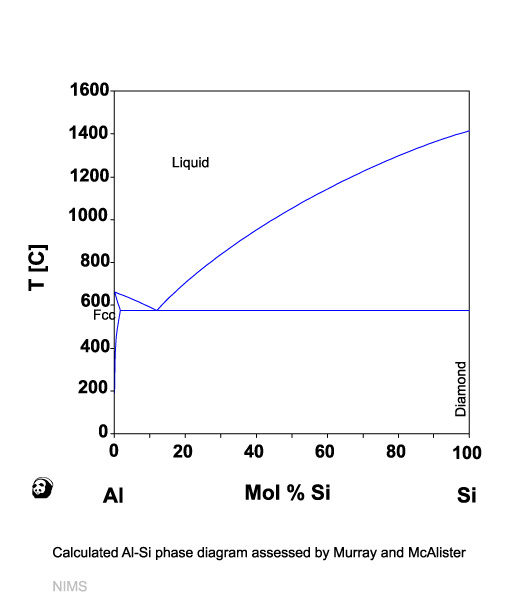
1. Obtain an estimate for the heat of fusion for the Al/Si eutectic (Joules per cm $^{3}$ of eutectic).
2. Calculate the bulk free energy gain (ignoring the energy associated with the Al/Si interfaces) associated with the solidification of 1 cm3 of eutectic at 560 °C.
3. Calculate the width of the Al and Si phases in a lamellar eutectic for the case where the total free energy change (including the energy associated with the interfaces) on solidification at 560 °C is equal to zero. Assume an interfacial free energy for the Al/Si interface of 350 mJ/m $^{2}$ .
4. Compare the phase widths from part c to the critical radii for the solidification of pure Al and pure Si at an undercooling of 20 $^{○}$ C. Assume that the solid liquid interfacial free energies are similar in magnitude to the Al/Si (solid/solid) interfacial free energy.
5. How good is the assumption of ideal liquid mixing in this case? Plot the liquidus lines for the Al-rich and Si-rich phases, using the equation that was developed in class. Compare the location of these lines with the location of the actual eutectic point, and comment on the agreement that you observe.

27.11 Eutectoid Transormations

Imagine the Fe-0.15 wt% C alloy in the figure below is austenitized above A 3 , and then quenched to800 ○ C where ferrite nucleates and covers the austenite grain boundaries.
1. Draw a composition profile normal to the $α / γ$ interface after partial transformation assuming diffusion-controlled growth.
1. Derive an approximate expression for the thickness of the ferrite slabs as a function of time.
The eutectoid temperature for the Fe/C phase diagram is 723 ○ C. Pearlite formed at 713 ○ C has a lamellar period ( λ ) of 1 μ m .
1. Calculate the lamellar period for pearlite that you would expect if the pearlite were formed at a temperature of 623 $^{○}$ C.
2. Pearlite forms initially at grain boundaries within the parent austenite phase. Briefly describe why this is so.
3. Describe what happens to the microstructure of the steel and to the hardness as increasingly large cooling rates are used. Discuss the role of carbon diffusion, and the role of both equilibrium and non-equilibrium phases.
In the reading about the Wright Flyer Crankcase, the authors assert “In an Al-Cu alloy with significant supersaturation, GP zones develop by spinodal decomposition. The spacing between zones (before coarsening) is determined by the fastest growing wavelength during decomposition. The favored wavelength is inversely related to the second derivative of the free energy versus composition function,which is zero at the spinodal line (located inside but near the GP zone solvus curve) and increases(negatively) with an increase in Cu or a decrease in temperature. Thus, the favored wavelength in the region with a large amount of Cu is smaller than in the regions with small amounts of Cu, and the resulting spacing between zones is smaller.”
1. Support their argument using the equations derived in class for spinodal decomposition. A good way to approach this is to postulate a spinodal line and then consider two cases, i.e. $X_{o} = 2.5$ wt.% Cu and $X_{o} = 4.5$ wt.% Cu, in detail, based on this spinodal. Be sure to also explain why the authors made the parenthetical statement “(before coarsening)”.
2. Is their argument entirely valid or do certain conditions need to be met? If so, what qualifications should be made to make it more accurate?
3. The authors claim that “The growth of [GP] zones is ultimately limited by solute depletion in the matrix. Despite its high solute concentration, the region with a large amount of Cu is depleted of solute by the time the zones have grown to about 10 nm.” Let's assume with them the GP zones grow at 100 $^{○}$ C from a matrix with 4.5 wt.% Cu. How do the authors arrive at this statement, what evidence did they likely use, and what calculations did they perform to arrive at this statement?

27.12 Transitional Phases

Suppose an alloy containing 97 wt. % aluminum and 3 wt. % copper is poured into a mold and solidified by extracting heat from the external surfaces of the mold.
1. What phase (or phases) do you expect to be present in the solid immediately after the solidification reaction?
1. What phase (or phases) will be present at equilibrium?
2. A variety of non-equilibrium phases are observed at intermediate stages in the transformation process. Why are these phases observed?
3. Once the equilibrium phase is formed, its rate of growth is found to decrease with time. Why is this? What is the rate limiting step in the transformation?
Porter and Easterling, prob. 5.6
Suppose that in the system of interest, $χ$ is inversely proportional to the absolute temperature, and the critical temperature for this system is 350 K. Replot the phase diagram from part a with temperature on the vertical axis.

27.13 TTT diagrams

Consider the following blowup of the low concentration region of a phase diagram similar to the Co-Cu diagram shown above:
1. At an average alloy composition $φ_{0}$ shown on this plot, it is determined that only $β$ precipitates form (no $γ$ is ever observed) at two temperatures, $T_{1}$ and $T_{2}$ . The time dependence of the appearance of $β$ is plotted at these two temperatures as shown below. On the plot above, indicate locations of $T_{1}$ and $T_{2}$ that are consistent with these curves, and briefly describe your reasoning.
1. Draw TTT curves for the precipitation of both $β$ and $γ$ for an alloy with the composition of $φ_{0}$ , making connections to specific temperatures from the phase diagram where possible.

27.14 Mineralization

Calculate the $C O_{3}^{2 -}$ concentration in equilibrium with seawater and with each of the following three forms of calcium carbonate: calcite, aragonite, vaterite. You'll need to use the solubility products provided in class, and look up the calcium concentration in seawater.

27.15 Review Questions

What does the liquid composition look like in front of an advancing solid phase?
What controls length scale of the composition variation?
What is the criteria for interface stability with respect to the formation of dendrites?
Under what conditions are dendrites formed during the solidification of a pure material?
What is the qualitative behavior of $S (θ)$ for nucleation at a flat interface, and at grain boundary surfaces, edges and corners?
How are equilibrium contact angles related to surface and interfacial free energies?
What is meant by complete wetting?
- What is the effect on nucleation for the complete wetting case?
What are the characteristic frequencies and concentrations ( $C_{0}, ν_{0}$ ) that determine the homogeneous and heterogeneous nucleation rates?
Why is coherent nucleation generally the favored homogeneous nucleation mechanism?
How is the work to form the critical nucleus calculated?
What is the 'incoherent solvus', and how does it relate to the expressions listed above?
Where does the Laplace pressure come from?
How do you know that kinetic factors must be controlling complex morphologies (dendrite formation, shapes of snowflakes, etc.)?
What controls the size of the depletion zone in front of a flat or curved precipitate that is growing?
How does it evolve with time?
What limits the growth velocity of a precipitate phase boundary at high and low temperatures?
- Which of these limits are connected to the phase diagram?
Why are flat, plate-like precipitates sometimes formed?
How does the molar free energy depend on the radius of curvature of a precipitate?
How does curvature effect the equilibrium concentration of solute that is in equilibrium with a precipitate?
What does the concentration dependence look like for precipitates that are larger than r*?
- What if the precipitate is smaller than r*?
What are transition phases, and why do they form?
- What is the mechanism by which transition phases shrink at the expense of equilibrium phases?
How are TTT curves for transition phases related to the phase diagram?
What are the basic physical assumptions of the Lifshitz/Slyosov coarsening theory discussed in class?
- What do the depletion zones look like?
- What determines the average solute concentration in the matrix phase?
What does the distribution of precipitates look like if coarsening occurs by the Lifshitz/Slyosov mechanism?
What do the binodal and spinodal curves look like for the regular solution model?
- What is the critical temperature?
What determines the size of the characteristic phase size when phase separation occurs by spinodal decomposition?
What is meant by uphill diffusion?
- When is it observed?
How is this phase size modified (in qualitative terms) by coherent strains?
How do these strains modify the phase diagram to give coherent spinodal and binodal curves?
How can the liquidus lines be estimated for an ideal eutectic system?
- What are the assumptions made in the approximation?
What determines the size of the individual phases for eutectic solidification?
What determines the size of the individual phases for a eutectoid transformation?
What is the physical significance of the squared gradient term in the free energy expression?
How can the shapes and sizes of metallic nanoparticles be controlled?
What is the growth mechanism of Si nanowires catalyzed by Gold?
- What is the importance of the Au/Si phase diagram.
How does the solubility of calcite compare to the solubility of aragonite or vaterite, and why?
- How is the concept of the solubility product used?
In the two-phase mixture of n-type and p-type materials used to form an organic solar cell, what sort of phase morphology is desired, and why?

28 316-2 Laboratories

28.1 Laboratory 1: Nucleation and Solidification in a Binary Eutectic Salt System

28.1.1 Laboratory Objectives:

To observe phase transformations in a binary eutectic system and the formation and subsequent coarsening of dendrites.

28.1.2 Learning Outcomes:

Upon completing the lab exercise, students should be able to:

Explain the observation of birefringence.
Discuss undercooling and observations related to cooling rate.
Quantify coarsening using measured secondary arm spacing and surface area to volume ratios. Predict how $S_{v}$ will change with coarsening.
Estimate uncertainty in measured values (temperature and dimension).

28.1.3 General Instructions:

Read through the lab before you begin. It is possible to acquire data for parts II and III during the same runs, but you must anticipate when to pause the temperature on the hotstage and when to acquire images on the printer. Parts I and II are measurements of phase transitions and dendrite growth rates and initial secondary arm spacing at a constant cooling rate. Part III is a measure of dendrite evolution as a function of time at a constant temperature. Therefore, you could pause the temperature of the system as soon as dendrites appear. The initial progression of the dendrite across the screen will provide you with the rate for part II; the subsequent evolution of the structure at a constant temperature will provide the data for part III. Note: setup a video file and record time / temperature / scale bar on the images.

Figure 28.1: Phase diagram for the ammonium nitrate/sodium nitrate system.

Part I: Solidification

Use the hotstage and transmission microscope to observe melting and solidification of

\sim

10wt% NaNO3 in the above salt system. Record transition temperatures on heating and cooling, and carefully note which transitions they correspond to. Fill in the table, below.

Table 2: Tempeartures of phase transformations at different cooling rates.

Rate		T(eut)	T( $δ - ϵ)$	T(liq)
	Heating
	Cooling
	Heating
	Cooling
	Heating
	Cooling

Birefringence: Are any of the phases observed during heating and cooling birefringent? Which? Label the phase diagram.

Part II: Observing the Microstructure as a Function of Constant Cooling Rate:

A. Cool the sample from the melt at a rate between 1 deg/ minute and 15 degrees per minute. Watch the melt (from the microscope – it has a larger area of view than the camera) until you observe the primary solidification begin, then “hold” the temperature and start recording the video image. The actual distance can be scaled based on the magnification, and the dendrite growth velocity calculated from these results. The information for Part III may be obtained by continuing to record as the microstructure evolves with time at constant temperature.

B. Repeat (A) for two additional cooling rates.

Table 3: Data collection table for constant cooling rate.

Rate	T (dendrite formation)	Dendrite growth rate*	**Initial secondary arm spacing ***

* Correct for magnification.

Magnification : ________________________

Part III: Observing the Microstructure as a Function of Time at Constant Temperature (Isothermal Experiments)

Repeat (A), but when solidification begins, pause the hotstage. Note the temperature. Capture images as a function of time (isothermal this time). Note: We will pause the temperature when we observe the dendrite formation. So the initial dendrite velocity, as well as the initial dendrite secondary arm spacing is a function of constant cooling rate; subsequent dendrite coarsening (secondary arm spacing) is a function of time at a constant temperature.

Table 4: Measured dendrite properties for isothermal experiments. Paused temperature = _____________.

Time	Secondary Arm Spacing	Surface Area to Volume Counts

Table 5: Measured dendrite properties for isothermal experiments. Paused temperature = _____________.

Time	Secondary Arm Spacing	Surface Area to Volume Counts

28.1.4 Lab Write Up:

Answer the following questions, using appropriate discussion of results, tables and plots. Neatness counts.

Describe what equipment was used in this lab and what measurements were made.
Make a table of your temperature results.
Is the temperature of the hotstage reliable? Why or why not? Be quantitative. Use your observations to substantiate your answer.
Did you observe birefringent phases? Which? Did you observe phases that were not birefringent? Which? What are the corresponding crystal structures?
Is there a relationship between the transition temperatures and the rate of cooling? What is it?
Does dendrite growth velocity depend on the cooling rate? What trend to you observe? Discuss.
From the constant cooling rate data, plot (initial) secondary arm spacing vs. cooling rate. Discuss.
Quantitatively, the secondary arm spacing is predicted to increase as a function of time to the 1/3 power. Plot the secondary arm spacing vs. time to determine if your data exhibits this behavior. Use the isothermal data.
The quantitative behavior of the surface area to volume ratio is predicted to change as time to the -1/3 power. What do your results indicate about coarsening? You can use overlays to determine the surface area per unit volume (# intersection of curved lines with phase / # points on overlay).
Choose a set of images, one taken at the initial dendrite formation, a second after some time has elapsed. Estimate the radius of curvature in each case. Assume that you had a uniform distribution of spheres, first with radius 1, coarsening to radius 2, using the two values above. Calculate the change in surface area to volume of such a change in radii. . Show your work. If you didn’t measure these, try to choose reasonable values. Approximate the radius of curvature of the tip by half the distance across a secondary dendrite arm.

28.2 Laboratory 2: Age Hardening in Al Alloys

28.2.1 Objective:

To determine the hardness and conductivity versus aging time of 2024 (1” wide x 1/8” thick), 6061 (1/2” wide x 1/8” thick) and 7075 (1” wide x ¼ “ thick) aluminum alloys aged at temperatures of 25°C, 125°C, 225°C. Each lab section will be responsible for a single alloy. Aging will be conducted over the course of the week; team members should plan to make measurements throughout the week.

28.2.2 Final write-up:

Data from the three lab sections will be pooled. This must be submitted by the end of week 2. Group reports will need to include (discuss) ALL class data.

28.2.3 Procedure:

Measure as-received, un-solutionized samples.

Alloy

Hardness Scale

Hardness (5 values)

Conductivity
Solution-treat~ a set samples of each alloy at 500C for one hour. Quench in ice water.
Measure the hardness of each solutionized sample (5 measurements on each!); discard outliers. Record.
Measure conductivity. Note: the sample MUST be at room temp. (do this after hardness) Record. Store samples in ice water.

Table 6: Hardness and Conductivity of Various Samples

Sample #

Hardness (5 values)

Conductivity
Anneal at:
1. room temperature
2. 125 °C
3. 225°C

for times ranging from 10 minutes, ½ hour, 1 hour, 2 hours….64, 128, 264 hours….Note that data will be plotted on a logarithmic scale. Use this information to plan your measurements.

Table 7:

Sample #	T ( $^{○}$ C)	Date in	Time in	Date out	Time out	Anneal time (min)	Hardness (5 meas)	$σ$ 5 meas)

28.2.4 Group report (informal)

First describe each alloy. (What do the 2XXX, 6XXX, and 7XXX designations indicate?) Give some examples of applications in each case. Indicate what the normal thermo-mechanical heat-treatments (tempers) would be for each alloy. Discuss your results in the context of these heat-treatments. (Include references.)

Plot hardness versus log-time for each of the temperatures measured using the pooled data.
Discuss the curves and their relative magnitudes and relative position on the time axis of any peaks observed, and label appropriately. In your own words, discuss in terms of the theory of precipitation hardening.
Plot conductivity vs. log-time. Correlate with hardness measurements. Why does the conductivity change?
Discuss uncertainties in your data. Include error bars on your figures. Use the correct number of significant figures. Assuming a normal (Gaussian) distribution of these values, you can find the uncertainty of the mean to within a 95% confidence level ,by determining 2X the standard error of the mean: 2x the standard deviation (STDEV in Excel) divided by the square root of the number of points measured (COUNT in Excel). There is a single command to do this: CONFIDENCE (.05, STDEV, COUNT). Indicate these values on your plots by adding error bars: left click the data set and choose Format data series > Y error bars. Note that you can use the Custom error bar command to add different values for each data point (i.e. each mean value of hardness for each individual sample).

Be sure to include the following:

Data from all alloys – not just the one measured by your group.
error bars on plots – see the handout.
results on as-received samples (Note that the 2024 samples had a T4 temper. The 6061 and 7075 samples had a T6 temper. Your discussion should define these, and indicate if they make sense, based on your aging results.)
results on solutionized samples.

References

Porter and Easterling [3], pages 291-308. Matter program (on Macs). Rosen paper posted on Bb, others you might find.

28.3 Laboratory 3: Al-Si Alloy Solidification and Modification (not currently used)

28.3.1 Experiment:

Each lab group (2-3 individuals) will prepare a castable alloy of AlSi using Al and a “Master Alloy” of 50wt% Al/Si. One group in each section should choose a hypoeutectic composition, another the hypereutectic composition, a third, if there is one, the eutectic composition. Consult the Al-Si phase diagram. Total alloy mass should be~ 25 grams. Once cast, we will cut a portion of this sample to polish, and a portion to re-cast with a 10%Sr, 90%Al alloy to achieve Sr compositions between .05 and .2 wt% Sr. We will examine the microstructures of the polished alloys.

28.3.2 Write-up (memo style):

Project objectives – brief summary. Why are Al-Si alloys of interest?
Methods – briefly summarize procedures.
Results and Discussion
- Micrographs:
  - Hypo, hyper and (if done) eutectic unmodified samples
  - Modified samples – compare to unmodified.
- Stereology
  - How do Image J results compare to predictions from phase diagram?
- Details of microscopy – is Jackson criteria valid?
- Other observations: porosity? Differences from center-to-edge of samples? What? Why?\

28.3.3 Experimental details (record here):

Mass Al:
Mass Al(50wt%)Si(50wt%) master alloy:
Alloy composition (wt% Si):
Mass of alloy used for modification:
Mass of Al(90wt%)Sr(10wt%): Note: Target amount = .05 - .2 wt% Sr
Other details, i.e furnace temperatures, materials, procedures used.

28.3.4 Short Answer Questions: due at the beginning of lab, week 2

We will be using the casting process in lab. What limitations or potential difficulties can you anticipate using this technique?
You have already used the AlSi phase diagram to predict the microstructure for each alloy. Can further detail be added? Can you predict any differences in primary phase formation? Use the Jackson criteria, discussed in P&E in section 3.4.6 (p. 170) to predict in detail what the shape of the primary phase in the hypo and hyper-eutectic alloys might be. Show your work. Lv, Si = 1788 kJ/kg; Lv, Al = 397 kJ/kg. Q – will the microstructures look like figure 3.65 (a) or (b) or neither?
How might the microstructure be further controlled by solidification conditions?
What might be the technological importance of Al-Si alloys?
What effect do modifiers (careful – “grain refiners” and “modifiers” play different roles) have on the microstructure?
Why is the modification in (6) desired?
A recent research summary by Napolitano et al. attributes the differences in morphology between un-modified and modified AlSi alloys to a variety of factors. Describe these factors.

References

1R. Jin, "Photoinduced Conversion of Silver Nanospheres to Nanoprisms", Science 294, 5548 (2001), pp. 1901--1903.

2K. G Libbrecht, "The Physics of Snow Crystals", Reports on Progress in Physics 68 (2005), pp. 855.

3David A Porter, K. E Easterling, and Mohamed Y Sherif, Phase Transformations in Metals and Alloys. (Boca Raton, FL: CRC Press, 2009).

4Y. Sun, "Shape-Controlled Synthesis of Gold and Silver Nanoparticles", Science 298, 5601 (2002), pp. 2176--2179.

5Andrea R. Tao, Susan Habas, and Peidong Yang, "Shape Control of Colloidal Metal Nanocrystals", Small 4, 3 (2008), pp. 310--325.

6Bozhi Tian, Xiaolin Zheng, Thomas J. Kempa, Ying Fang, Nanfang Yu, Guihua Yu, Jinlin Huang, and Charles M. Lieber, "Coaxial Silicon Nanowires as Solar Cells and Nanoelectronic Power Sources", Nature 449, 7164 (2007), pp. 885--889.

7D. Turnbull and R. E. Cech, "Microscopic Observation of the Solidification of Small Metal Droplets", Journal of Applied Physics 21, 8 (1950), pp. 804--810.

8Z. L. Wang, "Transmission Electron Microscopy of Shape-Controlled Nanocrystals and Their Assemblies", J. Phys. Chem. B 104, 6 (2000), pp. 1153--1175.

Time in hours	$X (t)$
0.4	0.08
0.7	0.10
1	0.14
2	0.17
4	0.23
6	0.28

Alloy	Hardness Scale	Hardness (5 values)	Conductivity

Sample #	Hardness (5 values)	Conductivity

316-2: Microstructural Dynamics II

Table of Contents

1 Catalog Description (316-1,2)

2 Course Outcomes

3 Introduction

4 Homogeneous Nucleation in Unary Systems

5 Kinetics of Homogeneous Nucleation in Unary Systems

6 Heterogeneous Nucleation in Unary Systems

7 Nucleation in Binary Systems

8 Strain Effects in Nucleation

9 Kinetics of Nucleation in the Solid State

10 Solidification in Unary Systems

11 Solidification in Binary Systems

12 Precipitate Growth

13 Growth and Curvature

14 Coarsening

15 Kinetics of Phase Transformations

16 Spinodal Decomposition

17 Case Study: Precipitation of Cu-rich Precipitates from Al:

18 Case Study: Mineralization from Solution

19 Case Study: Nanoparticle Nucleation and Growth

19.1 Motivation

19.2 Wulff Constuction

19.3 Kinetic Control of Particle Shape

19.4 Controlling Growth Rates

20 Interface Stability

21 Eutectic Solidification

Optimum phase size for eutectic microstructure:

22 Eutectoid Reactions

23 Review Questions

24 Matlab Example Scripts

24.1 Free energy of water droplets formed from water vapor at 10 K (Figure 4.2)

24.2 Laplace pressure, critical radius, and reversible work of nucleation for condensation of water from vapor, as a function of temperature (Figure 4.4)

24.3 General Nucleation Rate (Figure 5.2)

24.4 Nucleation Rate for Water Condensation (Figure 5.3)

24.5 Figure TOC entry

24.6 Figure TOC entry

24.7 Figure TOC entry

24.8 Figure TOC entry

24.9 Figure TOC entry

24.10 Figure TOC entry

24.11 Figure TOC entry

24.12 Figure TOC entry

24.13 Figure TOC entry

24.14 Figure TOC entry

24.15 Figure TOC entry

24.16 Figure TOC entry

24.17 Figure TOC entry

24.18 Figure TOC entry

24.19 Figure TOC entry

24.20 Figure TOC entry

25 Lab Examples

25.1 Coarsening

25.2 Secondary Arm Spacing

25.3 Surface to Volume Ratio

25.4 Temperature Dependence: K

25.5 LSW Theory

25.6 Estimating D

25.7 Estimating the Expected Coarsening Constant

25.8 Heat treatment of Al alloys

26 Appendix: Thermodynamic Data for Cu

27 316-2 Problems

27.1 General

27.2 Laplace Pressure Derivation

27.3 Homogeneous Nucleation

27.4 Surface and Interface Effects

27.5 Heterogeneous Nucleation

27.6 Nucleation in a Binary System

27.7 Spinodal Decomposition

27.8 Constitutional Undercooling and the 'Mushy Zone'

27.9 Coarsening

27.10 Eutectic Solidification

27.11 Eutectoid Transormations

27.12 Transitional Phases

27.13 TTT diagrams

27.14 Mineralization

27.15 Review Questions

28 316-2 Laboratories

28.1 Laboratory 1: Nucleation and Solidification in a Binary Eutectic Salt System

28.1.1 Laboratory Objectives: