332: Mechanical Behavior of Materials
Department of Materials Science and EngineeringNorthwestern University
1 Catalog Description
Plastic deformation and fracture of metals, ceramics, and polymeric materials; structure/property relations. Role of imperfections, state of stress, temperatures, strain rate. Lectures, laboratory. Prerequisites: 316 1; 316 2 (may be taken concurrently).
2 Course Outcomes
At the conclusion of the course students will be able to:
- Apply basic concepts of linear elasticity, including multiaxial stress-strain relationships through elastic constants for single and polycrystals.
- Quantify the different strengthening mechanisms in crystalline materials, based on interactions between dislocations and obstacles, such as: point defect (solid solution strengthening), dislocations (work hardening), grain boundaries (boundary strengthening) and particles (precipitation and dispersion strengthening).
- Apply fracture mechanics concepts to determine quantitatively when existing cracks in a material will grow.
- Describe how composite toughening mechanisms operate in ceramic matrix and polymer matrix composties.
- Derive simple relationships for the composite stiffness and strength based on those of the constituent phases.
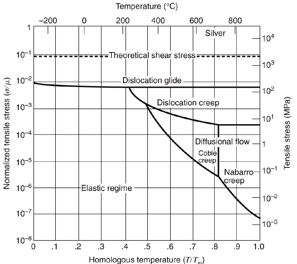
- Exhibit a quantitative understanding of high temperature deformation in metals and ceramics, based on various creep mechanisms relate to diffusional and dislocation flow (Coble, Nabarro-Herring and Dislocation creep/climb mechanisms).
- Exhibit a basic understanding of factors affecting fatigue in engineering materials, as related to crack nucleation and propagation, as well as their connection to macroscopic fatigue phenomena.
- Describe the interplay between surface phenomena (environmental attack) and stresses leading to material embrittlement.
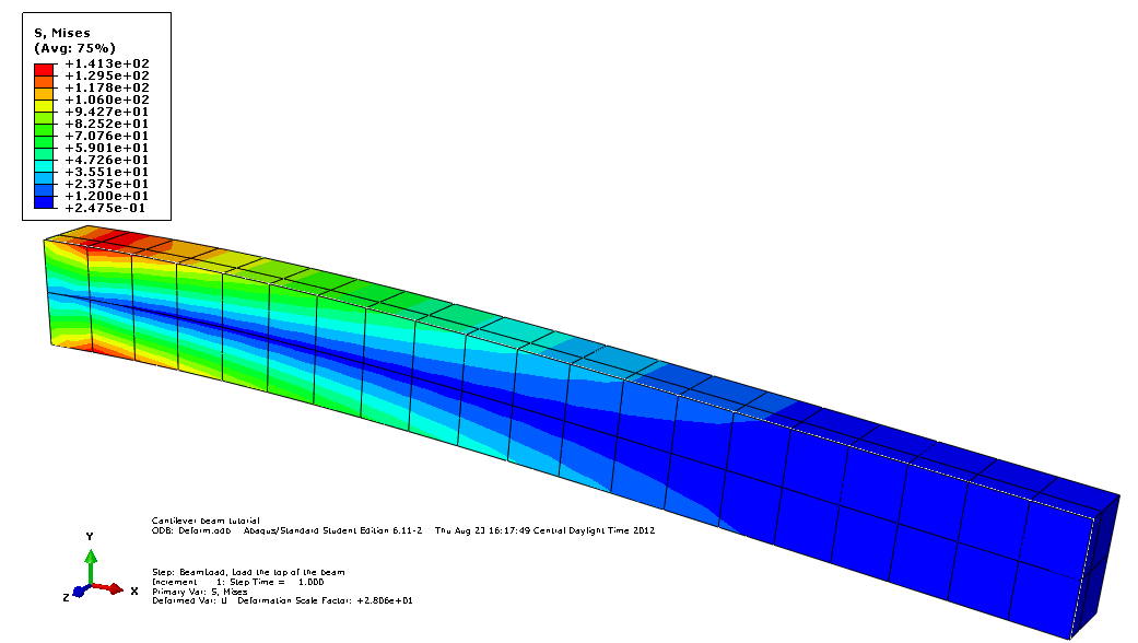
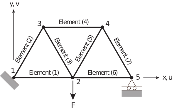
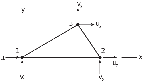
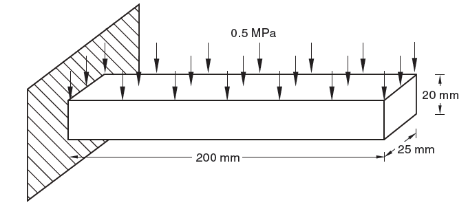
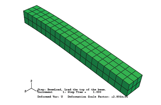
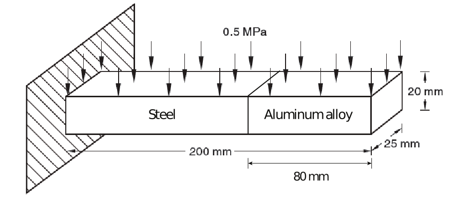
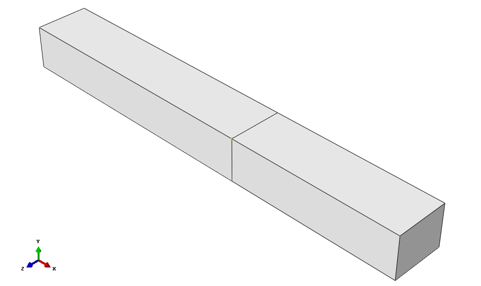
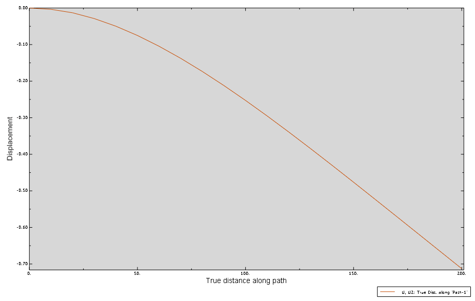
- Use the finite element method to calculate the stress and strain states for simple test cases, including a cantilever beam and a material with a circulat hole that is placed in tension.
- Use complex moduli to solve mechanics problems involving an oscillatory stress.
- Prepare and characterize specimens for measurement of mechanical properties.
- Write results from a laboratory project in the form of a journal article, and present their work orally as would be required in a technical forum.
- Select materials based on design requirements.
3 Introduction
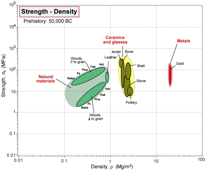
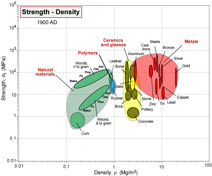
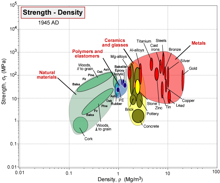
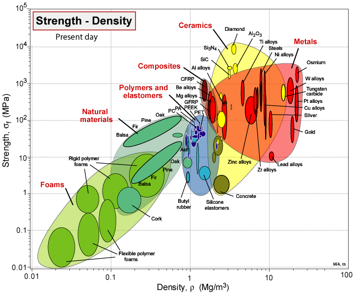
In Figure
3.1, we show the materials available to mankind from the beginning of time until the current day.[
3] The data are plotted as so-called 'Ashby plots', where two material properties are chosen for the x and y axes. In Figure
3.1 we use density to separate different materials along the x axis, and the fracture strength,
, to separate materials on the y axis. When the story begins, all we had to work with are the materials we could find around us or dig out of the ground. Over time, we Figure d out how to produce more materials for all kinds of purposes. The biggest developments come after World War II, a situation that coincides with the emergence of materials science as a discipline. We no longer rely on empiricism for materials development, but can actually begin to design new materials with the properties we want, or at least design materials that re better than anything we had before. The principles underlying the development of materials with the mechanical response forms the basis for this course.
4 Stress and Strain
The mechanical properties of a material are defined in terms of the strain response of material after a certain stress is applied. In order to properly understand mechanical properties, we have to have a good understanding of stress and strain, so that's where we begin.
Some Notes on Notation:
There are different ways to represent scalar quantities, vectors and matrices. Here's how we do it in this text:
- Scalar quantities are straight up symbols, like , , etc.
- Vectors are indicated with an arrow over the symbol, like .
- Unit vectors are indicated with a caret above the symbol, like
- Matrices are enclosed in square brackets, like
4.1 Tensor Representation of Stress
The
stress
applied to an object, which we denote as
or
is the force acting over an area of an object, divided by the area over which this force is acting. Note note that
is a matrix with individual components,
specified by the indices
and
. These indices have the following significance:
- i: surface normal (i= x, y, z)
- j: direction of force (j=x, y, z)
To obtain the
Engineering stress
,
, we use the undeformed areas of the stress-free object to obtain the stress tensor, whereas the true stress (which is what we generally mean when we write
) we use the actual areas in the as-stressed state.
The stress matrix is a
tensor
, which means that it obeys the coordinate transformation laws describe below. In two dimensions it has the following form:
The stress tensor must be symmetric, with
. If this were not the case, the torques on the volume element shown above in Figure
4.1 would not balance, and the material would not be in static equilibrium. As a result the two dimensional stress state is specified by three components of the stress tensor:
- 2 normal stresses, , . These are referred to as 'normal' stresses because the force acts perpendicular to the plane that it is referred to.
- A single shear stress, .
In three dimensions we add a axis to the existing and axes, so the stress state is defined by a symmetric 3x3 tensor. The full stress tensor can be used to define the stresses acting on any given plane. To simplify the notation a bit we label the three orthogonal directions by numbers (1, 2 and 3) instead of letters (, and ). The stress tensor gives the components of the force ( and ) acting on a given plane. The plane is specified by the orientation of the unit vector, that is perpendicular to the plane. This vector has components , and in the 1, 2 and 3 directions, respectively. It's a 'unit' vector because the length of the vector is 1, i.e. The relationship between , and is as follows:
or in more compact matrix notation:
Here
is the total cross sectional area of the plane that we are interested in. (If you need a refresher on matrix multiplication, the Wikipedia page on Matrix Multiplication (
https://en.wikipedia.org/wiki/Matrix_multiplication) [
16] is very helpful).
In graphical form the relationship is as shown in Figure
4.2. Like the 2-dimensional stress tensor mentioned above, the 3-dimensional stress tensor must also be symmetric in order for static equilibrium to be achieved. There are therefore 6 independent components of the three-dimensional stress tensor:
- 3 normal stresses, , and , describing stresses applied perpendicular to the 1, 2 and 3 faces of the cubic volume element.
- 3 shear stresses: , and .
The three dimensional stress tensor is a 3x3 matrix with 9 elements (though only 6 are independent), corresponding to the three stress components acting on each of the three orthogonal faces of cube in the Cartesian coordinate system used to define the stress components. The 1 face has
=1,
and
By setting
in Eq.
4.2, we get the following for the stresses acting on the 1 face of the volume element:
Equivalent expressions can be obtained for the stresses acting on the 2 and 3 faces, by setting and , respectively.
4.2 Tensor Transformation Law
The stress experienced by a material does not depend on the coordinate system used to define the stress state. The stress tensor will look very different if we chose a different set of coordinate axes to describe it, however, and it is important to understand how changing the coordinate system changes the stress tensor. We begin in this section by describing the procedure for obtaining the stress tensor that emerges from a given change in the coordinate system. We then describe the method for obtaining a specific set of coordinate axis which gives a diagonalized tensor where only normal stresses are present (Section
4.3).
4.2.1
Specification of the Transformation Matrix
In general, we consider the case where our 3 axes (which we refer to simply as axes 1, 2 and 3) are moved about the origin to define a new set of coordinate axes that we refer to as
,
and
. As an example, consider the simple counterclockwise rotation around the 3 axis by an angle
shown schematically in Figure
4.3. In general, the relative orientation of the transformed (rotated) and untransformed coordinate axes are given by a set of 9 angles between the 3 untransformed axes and the three transformed axes. In our notation we specify these angles as
, where
specifies the transformed axes (
,
or
) and
specifies the untransformed axis (1, 2 or 3). In our simple example, the angle between the 1 and
axes is
, so
. The angle between the 2 and
axes is also
, so
. The 3 axis remains unchanged in our rotation example, so
The
axis remains perpendicular to the 1,
, 2,
axes, so we have
Finally, we see that the angle between the
and the 2 axis is
(
) and the angle between the
and 1 axis is
(
). The full
matrix in this case is as follows:
Note that the matrix is NOT symmetric (), so you always need to make sure the first index, (denoting the row in the matrix) corresponds to the transformed axes, and the second index, (denoting the column in the matrix) corresponds to the original, untransformed axes.
4.2.2 Expressions for the Stress Components
Once we specify all the different components of , we can use the following general expression to obtain the stresses in the new (primed) coordinate system as a function of the stresses in the original coordinate system:
For each component of the stress tensor, we have to sum 9 individual terms (all combinations of and from 1 to 3). For example, is given as follows:
The calculation is breathtakingly tedious if we do it all by hand, so it makes sense to automate this and do the calculation via computer, in our case with Python. In this example we'll start with a simple stress state corresponding to uniaxial extension in the 1 direction, with the following untransformed stress tensor:
Suppose we want to obtain the stress tensor in the transformed coordinate system obtained from a 45
counterclockwise rotation around the z axis. The rotation matrix is given by Eq.
4.5, with
The following Python code solves for the full transformed tensor, with
given by Eq.
4.8 and
given by Eq.
4.5 with
:
#!/usr/bin/env python3
# -*- coding: utf-8 -*-
import numpy as np
sig=np.zeros((3, 3)) #% create stress tensor and set to zero
sig[0, 0] = 5e6; # this is the only nonzero component
sigp=np.zeros((3, 3)) # initalize rotated streses to zero
phi = 45
theta = [[phi,90-phi,90], [90+phi,phi,90], [90,90,0]]
theta = np.deg2rad(theta) # trig functions need angles in radians
for i in [0, 1, 2]:
for j in [0, 1, 2]:
for k in [0, 1, 2]:
for l in [0, 1, 2]:
sigp[i,j]=sigp[i,j]+np.cos(theta[i,k])*np.cos(theta[j,l])*sig[k,l]
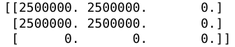
print(sigp) # display the transformed tensor components
We use Python because it is free, powerful, and quite easy to learn especially if you have experience with a similarly-structured programming environment like MATLAB. Various Python code examples are included in this text, and are presented as examples of how to do some useful things in Python.
The output generated by the Python code is shown in Figure
4.4, and corresponds to the following result:
Note the following:
- The normal stresses in the 1 and 2 directions are equal to one another.
- The transformed shear stress in the 1-2 plane is half the original tensile stress.
- The sum of the normal stresses (the sum of the diagonal components of the stress tensor) is unchanged by the coordinate transformation
4.2.3 An Easier Way: Transformation by Direct Matrix Multiplication
A much easier way to do the transformation is to use a little bit of matrix math. The approach we use is described in a very nice web page put together by Bob McGinty[
11]: A transformation matrix,
, is obtained by taking the cosines of all of these angles describing the relationship between the transformed and untransformed coordinate axes:
For the simple case of rotation about the z axis, the angles are given by Eq.
4.5, so that
is given as:
The transformed stress is now obtained by the following simple matrix multiplication:
where the is the transpose of:
For the rotation by around the z axis, is given by the following:
Equation
4.12 is much easier to deal with than Eq.
4.7. The Python code to take a uniaxial stress state and rotate the coordinate system by 45
about the 3 axis looks like this if we base it on Eq.
4.12:
import numpy as np

# create stress tensor with all zero elements
sig = np.zeros((3,3))

# set first one elment to be nonzero (one of the normal stresses)
sig[0][0] = 5e6

#set the rotation angle
phi = 45

# define the rotation matrix in degrees
theta = np.array([[phi,90+phi,90],[90-phi,phi,90],[90,90,0]])

# now put all the direction cosines in Q
Q = np.cos(np.radians(theta))

# claculate the transpose of Q
QT = np.transpose(Q)

# now multiply everything together
# note that we use the @ sign to multiply matrices in python
sigp = np.round(Q@sig@QT)

# print the result
print(sigp)
Running this script gives the output shown in Figure
4.4,
i.e. we obtain exactly the same result we obtained by using Eq.
4.7.
4.3 Principal Stresses
Any stress state (true stress) can be written in terms of three principal stresses
,
and
, applied in three perpendicular directions as illustrated in Figure
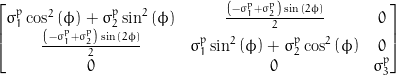
4.5. Note that we still need 6 independent parameters to specify a stress state: the 3 principal stresses, in addition to three parameters that specify the orientation of the principal axes. The stress tensor depends on our definition of the axes, but it is always possible to chose the axes so that all of the shear components of the stress tensor vanish, so that the stress tensor looks like the following:
In order to gain some insight into the points mentioned above, it is useful to consider a range of rotation angles, and not just a singe rotation angle of . One way to do this is to use the symbolic math capability of Python (or your other favorite software) to obtain the full stress tensor as a function of the rotation angle. We'll use the principal axes to define our untransformed state, and transform to a new set of axes by rotating counterclockwise by an angle around the 3 axis. We want to calculate
from Eqs.
4.11 and
4.12 as we did before, but we leave
as an independent variable. We use the following python script to do this:
# mohr_circle.py
# Mohr's circle derivation
from sympy import symbols, Matrix, cos, pi, simplify, preview

# specify the principal stressesS
sig1p, sig2p, sig3p = symbols(['sigma_1^p', 'sigma_2^p', 'sigma_3^p'])
sig = Matrix([[sig1p, 0, 0], [0, sig2p, 0], [0, 0, sig3p]])

# now specify the rotation angle
phi = symbols('phi')

# specify the theta matrix
theta=Matrix([[phi,pi/2-phi,pi/2], [pi/2+phi,phi,pi/2],[pi/2,pi/2,0]])

# take the cosine of all the elements in the matrix to get Q
Q=theta.applyfunc(cos)

# get the transpose of the matrix
QT=Q.transpose()

# now do the matrix multiplication to get the transformed matrix
sigp=Q*sig*QT

# now simplify and show the output
exp1 = simplify(sigp)
preview(exp1, filename='../figures/sympy_mohr_exp1.svg')

# define the center (C) and radius (R) of the circle
R, C = symbols(['R', 'C'])

# now we rewrite in terms of center and radius and simplify again
sigp = sigp.subs([(sig1p, C+R), (sig2p, C-R)])
exp2 = simplify(sigp)

# now save the exp1 and exp2 as image files
preview(exp1, viewer = 'file', filename = '../figures/sympy_mohr_exp1.png')
preview(exp2, viewer = 'file', filename = '../figures/sympy_mohr_exp2.png')
This results in the following expression for (exp1, generated in line 26 of mohr_circle.py).
This is not yet a very illuminating result, but it is the basis for the Mohr circle construction
, which provides a very useful way to visualize two dimensional stress states. This construction is described in more detail in the following Section.
4.3.1 Mohr's Circle Construction
The Mohr circle is a graphical construction that can be used to describe a two dimensional stress state. A two dimensional stress state is specified by two principal stresses, and , and by the orientation of the principal axes. The Mohr circle is drawn with a radius, , of , centered at on the horizontal axis. We can use these values of and as the independent variables in the expression for that we obtained from our python script. This substitution is made in lines 30-34 of mohr_circle.py, and leads to the following expression for (exp2 from line 34):
Python has taken us almost as far as we need to go, but it doesn't seem to be smart enough to use the following two trigonometric identities:
Substituting these into the expression for gives our final result:
In the Mohr circle construction normal stresses (
are plotted on the x axis and the shear component of the stress tensor
) is plotted on the y axis. For a two dimensional stress state in the 1-2 plane the circle is defined by two points:
and
. In our current example the stress state in the untransformed axes is represented by the open symbols in Figure
4.6,
i.e. by the points
and
. In the transformed axes the stress state is represented by the solid circles in Figure
4.6. From Eq.
4.17 it is evident that the relationship between the two different representations of the stress state is obtained by a rotation along circle by
. Whether this rotation is clockwise or counterclockwise depends on the sign convention in the definition of the shear stress. We're not going to worry about it here, but you can refer to the
Mohr's Circle Wikipedia article[
17] for the details (see the Section on the sign convention).
The Mohr circle construction can only be applied for a two dimensional meaning that there are no shear stresses with a component in the direction of the rotation axis. There can be a normal stress in the third direction, as in our example above, because this normal stress is simply superposed on the 2d stress state. In general, there are three principal stresses,
,
and
, and we can draw the Mohr circle construction with any combination of these 3 stresses. We end up with 3 different circles, as shown in Figure
4.7. Note that the convention is that
is the largest principal stress and that
is the smallest principal stress,
i.e. . An important result is that the largest shear stress,
, is given by the difference between the largest principal stress and the smallest one:
This maximum shear stress is an important quantity, because it determines when a material will deform plastically (much more on this later). In order to determine this maximum shear stress, we need to first Figure out what the principal stresses are. In some cases this is easy. In a uniaxial tensile test, one of the principals stresses is the applied stress, and the other two principal stresses are equal to zero.
The individual Mohr's circles in Figure
4.7 correspond to rotations in the around the individual principal axes. Circle
corresponds to rotation around the direction in which
is directed,
corresponds to rotation around the direction in which
is directed, and
corresponds to rotation around the direction in which
is directed. A consequence of this is that is always possible to use the Mohr's circle construction to determine the principal stresses if there is only one non-zero shear stress.
4.3.1.1 Exercise:
Determine the maximum shear stress for the following stress state:
4.3.1.2 Solution:
We can handle this one without using a computer. There is only one non-zero shear stress (), so we can determine the principals stresses in the following manner:
- One of the three principal stresses is the normal stress in the direction that does not involve either of the directions in the nonzero shear stress. Since the non-zero shear stress in our example is one of the principal stresses is =3 MPa.
- Now we draw a Mohr circle construction using the two normal stresses and the non-zero shear stress, in this case , and . Mohr's circle is centered at the the average of these two normal stresses, in our case at = 4 MPa.
- Determine the radius of the circle, , is given as:
- The principal stresses are given by the intersections of the circle with the horizontal axis:
The third principal stress is 3 MPa, as we already determined.
- The maximum shear stress is half the difference between the largest principal stress (6.64 MPa) and the smallest one (1.76), or 2.24 MPa.
4.3.2 Critical Resolved Shear Stress for Uniaxial Tension
As an example of the Mohr circle construction we can consider the calculation of the resolved shear stress on a sample in a state of uniaxial tension. The Mohr's circle representation of the stress state is shown in Figure
4.8. The resolved shear stress,
, for sample in uniaxial tension is given by the following expression:
where
is the applied tensile stress,
is the angle between the tensile axis and a vector normal to the plane of interest, and
is the angle between the tensile axis and the direction of the shear stress. This shear stress has to be in the plane itself, so for a 2-dimensional sample
. This means we can rewrite Eq.
4.20 in the following way:
We can use the identities and to obtain the following:
We can get the same thing from the Mohr's circle construction to redefine the axes by a rotation of . The shear stress is simply the radius of the circle ( in this case) multiplied by . Mohr's circle also gives us the normal stresses:
The untransformed 2-dimensional stress tensor looks like this:
The transformed stress tensor (after rotation by to give the resolved shear stress) looks like this:
4.3.3 Principal Stress Calculation
Principal stresses can easily by calculated for any stress state just by obtaining the eigenvalues
of the stress tensor. In addition, the orientation of the principal axes (the coordinate system for which there are no off-diagonal components in the stress tensor). If you need a refresher on what eigenvalues and eigenvectors actually are, take a look at the appropriate Wikipedia page (
http://en.wikipedia.org/wiki/Eigenvalues_and_eigenvectors). We'll use Python to do this, using the 'eig' command .
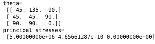
To illustrate, we'll start with the stress state specified by Eq.
4.9. which we got by starting with a simple uniaxial extension in the 1 direction, and rotating the coordinate system by 45
about the 3 axis. The MATLAB script to do this is very simple and is as follows:
#!/usr/bin/env python3
# -*- coding: utf-8 -*-

import numpy as np

# write down the stress tensor that we need to diagonalize
sig=1e6*np.array([[2.5,2.5,0],[2.5,2.5,0],[0,0,0]])

# get the eigen values and eigen vectors
[principalstresses, directions]=np.linalg.eig(sig)

# the columns in 'directions' correspond to the dot product of the
# principal axes with the orignal coordinate system
# The rotation angles are obtained by calculating the inverse cosines
theta=np.arccos(directions)*180/(np.pi)

# print the results (or just look at them in the variable explorer in Spyder)
print ('theta=\n', theta)
print ('principal stresses=\n', principalstresses)
Here's the output generated by this script:
3 principal axes returned as column vectors. In this case there is a single normal stress, acting in a direction midway between the original x and y axes. The original uniaxial stress state is recovered in this example, as it should be. To summarize:
- Principal Stresses: Eigenvalues of the stress tensor
- Principal Stress directions: Eigenvectors of the stress tensor
4.3.4 Stress Invariants
Some quantities are invariant to choice of axes. The most important one is the
,
, given by summing the diagonal components of the stress tensor and dividing by 3:
The negative sign appears because a positive pressure is compressive, but positive stresses are tensile. The hydrostatic pressure is closely related to a quantity referred to as the 'first
stress invariant',
:
The second and third stress invariants, and , are also independent of the way the axes are defined:
It's not obvious at first that each of these quantities are invariant to the choice of coordinate axes. As a check, we can start with a general tensor, rotate the coordinate system through a full 180 degrees, and plot the value of an invariant as a function of a the rotation angle, . The following python code does this for :
import numpy as np
import matplotlib.pyplot as plt

# create a function that multiplies the transforms a stress
# tensor sig by a rotation of phi about the Z axis,
# and returns the vaalue of I2

def I2_calc(phi):
    sig = np.array([[3, 5, 4], [5, 2, 9], [4, 9, 6]])
    theta = np.array([[phi,90+phi,90],[90-phi,phi,90],[90,90,0]])
    Q = np.cos(np.radians(theta))
    QT = np.transpose(Q)
    sigp = Q@sig@QT
    I2 = (sigp[0][0]*sigp[1][1]+sigp[1][1]*sigp[2][2]+sigp[2][2]*sigp[0][0]-
          sigp[0][1]**2 - sigp[1][2]**2 -sigp[0][2]**2)
    return I2

# vectorize the function so we can input an array of phi values
vI2 = np.vectorize(I2_calc)

# now calculate I2 over a range of phi values
phi = np.linspace(0, 180, 100)
I2vals = vI2(phi)

# now make the plot
plt.close('all')
fig, ax = plt.subplots(1,1, figsize=(3,3), constrained_layout=True)
ax.plot(phi, I2vals, '-')
ax.set_xlabel(r'$\phi (deg.)$')
ax.set_ylabel(r'$I_2$')

# save the plot
fig.savefig('../figures/I2plot.svg')
This results in the very boring plot shown in Figure
4.10, indicating that
really is invariant to the definition of the coordinate axes.
4.4 Strain
There are 3 related definitions of the strain:
- Engineering strain
- Tensor strain
- Generalized strain (large deformations, also referred to as 'finite strain')
Each of these definitions of strain describe the way different points an object move relative to one another when the material is deformed. Consider two points
and
, separated initially by the increments d
, d
and d
along the
,
and
directions. After the deformation is applied, these points move by the following amounts, as illustrated in Figure
4.11:
- moves by an amount
- moves by
4.4.1 Small Strains
Strain describes how much farther point to moved in three different directions, as a function of how far was from initially. For small strains we can ignore higher order terms in a Taylor expansion for , and and maintain only the first, partial derivative terms as follows:
The three normal components of the strain correspond to the change in the displacement in a given direction corresponds to a change in initial separation between the points of interest in the same direction:
The engineering shear strains are defined as follows:
Note: shear strains are often represented by the lower case Greek gamma to distinguish them from normal strains:
4.4.2 Tensor Shear Strains
Engineering strains relate two vectors to one another, () and (), just as a tensor does, but the the transformation law between different coordinate systems is not obeyed for the engineering strains. For this reason the engineering strains are NOT tensor strains. Fortunately, all we need to do to change engineering strains to tensor strains is to divide the shear components by 2. In our notation we use to indicate engineering strain and to indicate tensor strains. The tensor normal strains are exactly the same as the engineering normal strains:
Engineering shear strains () are divided by two to give tensor shear strains:
Note that the tensor strains must be used in coordinate transformations (axis rotation, calculation of principal strains, , , ).
4.4.3 Generalized Strain
We can also define the strain by considering a cube of side
that is deformed into a parallelepiped with dimensions of (along principal strain axes). After deformation, the cube has dimensions of
,
,
. Alternatively, a sphere of radius
is deformed into and ellipsoid with principal axes of
,
and
, as shown in Figure
4.12. The quantities
,
,
are
extension ratios
, and are related to the principal strains as follows:
The true strains
,
, are obtained as by taking the natural log of the relevant extension ratio. For example, for a uniaxial tensile test, the true strain in the tensile direction (assumed to be the 1 direction here) is:
This expression for the true strain can be obtained by recognizing that the incremental strain is always given by the fractional increase in length , where is the current length of the material as it is being deformed. If the initial length is and the final, deformed length is , then the total true strain, is obtained by integrating the incremental strains accumulated throughout the entire deformation history:
The extension ratios provide a useful description of the strain for both small and large values of the strain. A material with isotropic mechanical properties has the same coordinate axes for the principal stresses and the principal strains.
A more detailed description of generalized strain, with a lot of relevant matrix math, is provided in the Wikipedia article on finite strain theory (
https://en.wikipedia.org/wiki/Finite_strain_theory). This information is not needed for this class, but the reference is provided here as a useful resource for large strain. If you come across concepts like the
Cauchy-Green deformation tensor
or the
Finger deformation tensor
, this article provides a useful introduction (but prepared for a lot of matrix math). These concepts appear in a range of useful description of mechanical response, including many in the biomedical field (muscle actuation, deformation of skin, etc).
4.5 Deformation Modes
Now that we've formally defined stress and strain we can give some specific examples where these definitions are used, and begin to define some elastic constants. We'll begin with the two most fundamental deformation states: simple shear and hydrostatic compression. These are complementary strain states - for an isotropic material simple shear changes the shape but not the volume, and hydrostatic compression changes the volume but not the shape. We'll eventually show that for an isotropic material there are only two independent elastic constants, so if we know how an isotropic material behaves in response to these two stress states, we have a complete understanding of the elastic properties of the material.
4.5.1 Simple Shear
Simple shear
is a two dimensional strain state, which means that one of the principal strains is zero (or one of the principal extension ratios is 1).
The stress tensor looks like this:
From the definition of the engineering shear strain (Eq.
4.32) we have:
We need to divide the engineering shear strains by 2 to get the tensor strains, so we get the following:
We're generally going to use engineering strains and not tensor strains, so we generally don't need to worry about the factor of two. The exception is when we want to use a coordinate transformation to find the principal strains. To do this we use a procedure exactly analogous to the procedure described in Section
4.3, but we need to make sure we are using the tensor strains when we do the calculation.
The
shear modulus
is simply the ratio of the shear stress to the shear strain.
Note that the volume of the material is not changed, but it's shape has. In very general terms we can view the shear modulus of a material as a measure of its resistance to a change in shape under conditions where the volume remains constant.
4.5.2 Simple Shear and the Mohr's Circle Construction for Strains
Mohr's cirlcle
for strain looks just like Mohr's circle for stress, provided that we use the appropriate tensor components. That means that we need to plot
on the vertical axis and the normal strains on the vertical axis, as shown in Figure
4.14 (where we have used the common notation for the simple shear geometry, with
). One thing that we notice from this plot is that
is simply given by the difference between the two principal strains:
For simple shear this relationship is valid, even for large strains, even though there are other aspects of the Mohr's circle construction that no longer work at large strains. The primary difficulty is that the frame of reference for the strained and unstrained case are not the same. In general, strains rotate the frame of reference by an amount that we don't want to worry about for the purposes of this course. For small strains typically obtained in metals or ceramics (with strain amplitudes of a few percent or less) we don't need to worry about this rotation, but it can become important for polymeric systems that undergo very large strains prior to failure. However, if all we want a measure of the shear strain in the material, we can still use Eq.
4.43, regardless of how large the principal strains (and corresponding extension ratios) actually are.
I
4.5.3 Torsion
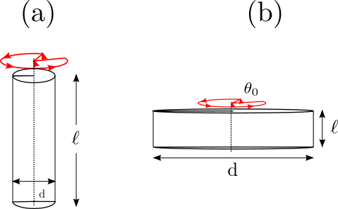
An important geometry for characterizing the shear properties of soft materials is the torsional geometry shown in Figure
4.15. In this material a cylindrical or disk-shaped material is twisted about an axis of symmetry. The material could be a long, thin fiber (Figure
4.15a) or a flat disk sandwiched between two plates (Figure
4.15b). We obtain the shear modulus by looking at the torsional stiffness of material,
, the Torque,
, required to rotate the top and bottom of the fiber by an angle
.
We define a cylindrical system with a z axis along the fiber axis. The other axes in this coordinate system are the distance from this axis of symmetry, and the angle around the z axis. The shear strain in the plane depends only on , and is given by:
The corresponding shear stress is obtained by multiplying by the shear modulus, :
We integrate the shear stress to give the torque, :
This geometry is commonly used in an oscillatory mode, where is oscillated at a specified frequency. In this case the torque response is obtained by using the dynamic shear modulus, (defined in the section on viscoelasticity) in place of .
4.5.4 Hydrostatic Compression
The
,
, of a material describes its resistance to a change in density. Formally, it is defined in terms of the dependence of the volume of the material on the hydrostatic pressure,
:
The hydrostatic stress state corresponds to the stress state where there are no shear stresses, and each of the normal stresses are equal. Compressive stresses are defined as negative, whereas a compressive pressure is positive, so the stress state for hydrostatic compression looks like this:
4.5.5 Uniaxial Extension
Uniaxial extension corresponds to the application of a normal stress along one direction, which we define here as the 3 direction so that the stress tensor looks like this:
We can measure two separate strains from this experiment: the longitudinal strain in the same direction that we apply the stress, and the transverse strain, , measured in the direction perpendicular to the applied stress (we'll assume that the sample is isotropic in the 1-2 plane, so . The strains are given by the fractional changes in the length and width of the sample:
From these strains we can define
,
, and
,
:
4.5.6 Longitudinal Compression
A final deformation state that we will consider is longitudinal compression. In this state all of the compression is in one direction, which we will specify as the 3 direction. The strains in the other two direction are constrained to be zero, so the strain state is as follows:
Note that the strain state is similar to that of uniaxial extension or compression (Figure
4.17), but in the current case we have a single nonzero strain instead of a single non-zero stress. Finite values of
and
must exist in order for sample in order for this strain state to be maintained, but we're not going to worry about those for now. Instead, we'll use the following relationship for the longitudinal elastic modulus,
which is the ratio of
to
for this strain state. Note that this deformation state changes both the shape and volume of the material, so
involves both
and
:
4.6 Representative Moduli
A few typical values for
and
are listed in Table
elsewhere. Liquids do not have a shear modulus, but they do have a bulk modulus.
Table 1: Representative elastic moduli for different materials.
|
Material
|
(Pa)
|
(Pa)
|
|
Air
|
0
|
1.0x10
|
|
Water
|
0
|
2.2x10
|
|
Jello
|
|
2.2x10
|
|
Plastic
|
|
2x10
|
|
Steel
|
8x10
|
1.6x10
|
4.7 Case Study: Speed of Sound
The speed of sound, or
sound velocity
,
, is actually a mechanical property. It is related to a modulus,
, in the following way:
Here is the density of the material. The modulus that we need to use depends on the type of sound wave that is propagating. The two most common are a shear wave and a longitudinal compressional wave:
- Longitudinal compressional wave:
- Shear wave:
In a liquid or gas (like air), and shear waves cannot propagate. In this case there is a single sound velocity obtained by setting . For an ideal gas:
If the compression is applied slowly enough so that the temperature of the gas can equilibrate, we have:
So we expect that for a gas, the compressive modulus just equal to the pressure. The situation is a bit more complicated for gas, since we need to use the adiabatic modulus, which is about 40% higher than the pressure itself. (For a detailed explanation, see the Wikipedia article on the speed of sound (
http://en.wikipedia.org/wiki/Speed_of_sound)[
20]. The brief explanation is that for sound propagation, the derivative in Eq.
4.57 needs to be evaluated at constant entropy and not constant temperature, because the sound oscillation is so fast that the heat does not have time to escape). With
=1.2 kg/m
and
Pa, we end up with a sound velocity of 344 m/s.
5 Matrix representation of Stress and Strain
As usual, we begin by replacing the directions (x, y, and z) with numbers:
,
,
. Once we do this we have 6 stress components, and six strain components. We then number these components from 1-6, so that 1, 2 and 3 are the normal components and 4, 5 and 6 are the shear components. We do this for both stress and strain as shown in Table
2.
Table 2: Definition of the matrix components of stress and strain.
|
Engineering stress
|
Matrix Stress
|
Engineering Strain
|
Matrix Strain
|
|
|
|
|
|
|
|
|
|
|
|
|
|
|
|
|
|
|
|
|
|
|
|
|
|
|
|
|
|
|
A series of elastic constants relate the stresses to the strains. We can do calculations in either of the following two ways:
- Start with a column vector consisting of the 6 elements of an applied stress, and use the compliance matrix to calculate the strains.
- Start with a column vector consisting of the 6 elements of an applied strain, and use the stiffness matrix to calculate the stresses.
In each case we use a matrix to relate two 6-element column vectors to one another. The procedure in each case is outlined below.
5.1 Compliance matrix
The matrix must be symmetric, with , so there are a maximum of 21 independent compliance coefficients:
Note that the compliance coefficients have the units of an inverse stress (Pa).
5.2 Stiffness Matrix
The stiffness matrix (c) is the inverse of compliance matrix (note the somewhat confusing notation in that the compliance matrix is and the stiffness is , backwards from what you might expect). The stiffness coefficients have units of stress.
5.3 Symmetry requirements on the compliance (or stiffness) matrix.
5.3.1 Orthorhombic symmetry
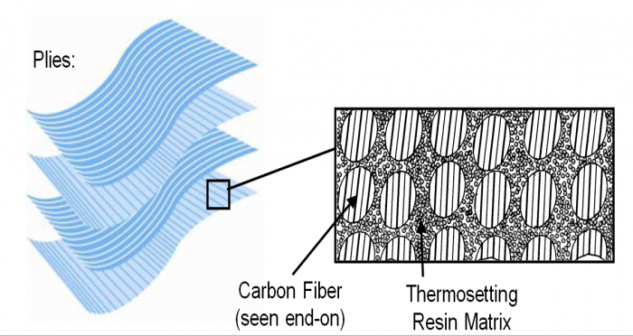
Extruded polymer sheets, like the one shown schematically in Figure
5.1 have orthorhombic symmetry, with different elastic properties in the extrusion, thickness and width directions. These materials have orthorhombic symmetry.
For materials with orthorhombic symmetry, the principal axes of stress and strain are identical, and all compliance components relating a shear strain (e
4, e
5 or e
6) to normal stresses (
,
or
) or to another shear stress must be zero. The stiffness matrix is as shown in Eq.
5.4 below, and there are 9 independent elastic constants. These 9 elastic constants can be identified as follows:
- , and , Young's moduli for extension in the 1, 2 and 3 directions, respectively.
- , and , Shear moduli for shear in the planes perpendicular to the 1, 2 and 3 directions, respectively.
- , and , which relate stresses in one direction to strains in the perpendicular direction.
5.3.2 Fiber Symmetry
For a material with fiber symmetry, one of the axes is unique (in this case the 3 axis) and the material is isotropic in the orthogonal plane. Since the 1 and 2 axes are identical, there are now 5 independent elastic constants , , , , :
Examples of materials with fiber symmetry include the following:
- Many liquid crystalline polymers (e.g. Kevlar).
- Materials after cold drawing (plastic deformation to high strains, carried out below the glass transition temperature or melting temperature of the material.)
To better understand the significance of the 5 elastic constants for fiber symmetry, it is useful to consider the types of experiment we would need to conduct to measure each of them for a cylindrical fiber. The necessary experiments are described below.
5.3.2.1 Fiber extension along 3 direction: measurement of and
We obtain
and
by performing a tensile test along the fiber axis (the 3 direction) as shown in Figure
5.2. The strain in the 3 direction is given by the fractional change in the length of the fiber after application of the load, and the strains in the 1 and 2 directions are given by the fractional changes in the diameter of the fiber:
We then obtain
and
from Eq.
5.5, recalling that
is the only non-zero stress component in this situation:
5.3.2.2 Fiber Torsion: Measurement of
We obtain the shear modulus by looking at the torsional stiffness of the fiber,
, the torque,
, required to rotate the top and bottom of the fiber by an angle
, as illustrated in Figure
5.3We define a cylindrical system with a z axis along the fiber axis. The other axes in this coordinate system are the distance from this axis of symmetry, and the angle around the z axis. The shear strain in the plane depends only on, and is given by :
The corresponding shear stress is obtained by multiplying by the shear modulus, characterizing deformation in the 1-2 and 2-3 planes:
We integrate the shear stress to give the torque, :
So once we know the torsional stiffness of the fiber (the relationship between the applied and we know the shear modulus, . This shear modulus is simply the inverse of:
5.3.3 Fiber compression in 1-2 plane: determination of and
The last two elastic constants for a material with fiber symmetry can be determined from an experiment where the fiber is confined between two surfaces and compressed as shown in Figure
5.4. The elastic constants can be determined by measuring the width of the contact region between the fiber and the confining surface. If the confining surfaces are much stiffer than the fiber itself, than this contact width,
, is determined by the elastic deformation of the material in the 1-2 plane. If there is no friction between the fiber and the confining surfaces the fiber is allowed to extend in the 3 direction as it is compressed and the contact width is given by the following expression:
where is the force applied to the fiber, is its undeformed diameter and is its length.
A practical situation that is often observed is that friction between the fiber and confining surfaces keeps the fiber length from increasing, so the strain in the three direction must be zero. If we express the stress state in terms of the principle stresses in 1 and 2 directions, we have the following from Eq.
5.5:
Setting to zero in this equation gives the following for :
A consequence of this stress is that the frictionless expression for gets modified to the following:
The remaining constant, , is determined from a measurement of , the ratio of the fiber width at the midplane to the original width of the fiber. This relationship is complicated, and involves several of the different elastic constants.
5.3.4 Cubic Symmetry
For a material with cubic symmetry the 1,2 and 3 axes are all identical to one another, and we end up with 3 independent elastic constants:
5.3.5 Isotropic systems
For an isotropic material all axes are equivalent, and the properties are invariant to any rotation of the coordinate axes. In this case there are two independent elastic constants, and the compliance matrix looks like this:
The requirement that the material properties be invariant with respect to any rotation of the coordinate axes results in the requirement that , so there are two independent elastic constants. The shear modulus, , Young's modulus and Poisson's ratio, are given as follows:
5.3.5.1 Bulk Modulus for an Isotropic Material
The bulk modulus, , of a material describes it's resistance to a change in volume (or density) when we apply a hydrostatic pressure, . It is defined in the following way:
The stress state in this case is as follows:
From the compliance matrix (Eq.
5.18) we get
. The change in volume,
can be written in terms of the three principal extension ratios,
,
and
:
Now we use the fact that for small , , so we have:
Recognizing that the derivative in the definition of can be written as the limit of for very small allows us to obtain the expression we want for :
5.3.5.2 Relationship between the Isotropic Elastic Constants:
Because there are only two independent elastic constants for an isotropic system and can be expressed in terms of some combination of and . For the relevant relationship is as follows.
We can also equate the two expressions for
in Eq.
5.25 to get the following expression for
:
Note that if , and .
5.3.6 Relationship between Stiffness Matrix and Compliance Matrix
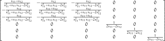
The stiffness matrix is the inverse of the compliance matrix. The relationships between the individual coefficients is quite complicated, unless there is a lot of symmetry. It's not too bad for the isotropic case, in which case we can use symbolic python to do the inversion. Here's the code:
from sympy import symbols, Matrix, preview
# specify two independent elements of s for an isotropic material
s11, s12 = symbols(['s_11', 's_12'])

# define the matrix
s = Matrix([[s11, s12, s12, 0,0,0],
           [s12,s11,s12,0,0,0],
           [s12,s12,s11,0,0,0],
           [0,0,0,2*(s11-s12),0,0],
           [0,0,0,0,2*(s11-s12),0],
           [0,0,0,0,0,2*(s11-s12)]])

# now invert the matrix
c=s.inv()
preview(c, viewer = 'file', filename = '../figures/sympy_c.png')
This gives the output shown here:
Note that the stiffness matrix has the same symmetry as the compliance matrix, as it must:
Comparison of Eq.
5.27 to the output from symbolic_cmatrix.py gives the following:
6 Other Symmetry-Related Constitutive Relationships
Elasticity is just one of many properties that relate some sort of field (like stress) to a response (like the strain). A range of other properties also exist, with different properties defined by the same sort of symmetry relationships described above. Some of these are listed below in Table
3. A symmetry map that relates the appropriate property coefficients for these different cases is shown in Figure
6.1. Here we show 3 of these symmetry maps corresponding to 3 of 32 symmetry classes for materials. These are discussed in more detail in 361, but the concept is introduced here because it relates to the linear elastic properties.
|
Property
|
Symbol
|
Field (row)
|
Response (column)
|
|
tensor properties of rank 0 (scalars)
|
|
specific heat
|
(1x1)
|
|
|
|
tensor properties of rank 1 (vectors)
|
|
pyroelectricity
|
(3x1)
|
|
(electric displacement)
|
|
tensor properties of rank 2
|
|
Thermal expansion
|
(6x1)
|
|
|
|
Dielectric permittivity
|
(3x3)
|
(elec. field)
|
(electric displacement)
|
|
Electrical conductivity
|
(3x3)
|
|
(current density)
|
|
Thermoelectricity
|
(3x3)
|
(Temp. gradient)
|
(electric field)
|
|
tensor properties of rank 3
|
|
Piezoelectricity
|
(3x6)
|
(stress)
|
(electric displacement)
|
|
Converse piezeoelectricty
|
(6x3)
|
(elec. field)
|
(strain)
|
|
tensor properties of rank 4
|
|
Elasticity
|
(6x6)
|
|
|
Table 3: Some symmetry-related properties.
7 Contact Mechanics
In a simple tensile test involving a sample with a uniform cross section, the stresses and strains are both uniform throughout the entire sample. In almost any real application where we care about mechanical properties, this is not the case however. A simple example of this is the case where we press a rigid, cylinder into s soft, compliant material as shown in Figure
7.1.
7.1 Sign conventions
Sign conventions have a tendency to lead to confusion. This issue is particularly problematics in contact mechanics because compressive loads are considered to be positive, but a compressive stress is negative. Here's a summary of the sign conventions relevant to our treatment of contact mechanics:
- (force): a positive force is compressive
- (displacement): a positive displacement is compressive
- (stress): a positive stress is tensile
- (strain): a positive strain is tensile
In order not to get too hung up in issues related to the sign, we define and as the tensile loads and displacements:
7.2 Flat Punch Indentation
(Note: Many of issues presented here are discussed in more detail in a published review article: see ref.[
13]).
Consider a flat-ended cylindrical punch with a radius of
in contact with another material of thickness,
, as shown schematically in Figure
7.2. The material being indented by a punch rests on a rigid substrate. We are interested in the compressive force,
, that accompanies a compressive displacement,
, applied to the indenter.
7.2.1 Flat Punch: Approximate Result for an elastic half space.
For an elastic half space (), the strain field under the indenter is nonuniform. The largest strains are confined to a region with characteristic dimensions defined by the punch radius, . We can get a very approximate expression for the relationship between the compressive load, , and the compressive displacement, from the following approximate concepts:
- The average strain in the highly deformed region of the sample must increase linearly with . Because strain is dimensionless we need to divide by some length scale in the problem to get a strain. For an elastic half space with the only length scale in the problem is the punch radius, . So the strain fields must depend on . We'll take this one step further and assume that is an average in a region of volume under the punch:
- The average contact stress, under the punch can be quantitatively defined by dividing the compressive load by the stress:
- An approximate relationship between and is obtained by assuming that the stress and strain are related through the elastic modulus, i.e. . Using the equations above for the compliance, :
7.2.2 Flat punch - Detailed Result
In a more general situation both of the contacting materials (the indenter and the substrate) may deform to some extent, so the compliance depends on the properties of both materials. If the materials have Young's moduli of and and Poisson's ratios of and , then the expression for is:
where
is the following
reduced modulus
:
Note that for a stiff indenter, we have . This is the plane strain modulus that appears in a variety of situations, which we derive below.
7.2.3 Plane strain modulus.
The plane strain modulus, , describes the response of a material when it cannot contract in one of the directions that is perpendicular to an applied tensile stress. It's easy to derive this by using the compliance matrix for an amorphous material, which must look like this;
In writing the compliance matrix this way, we have used the fact that Young's modulus is and the Poisson's ratio is so we have and . Suppose we apply a stress in the 1 direction, and require that the strain in the 2 direction is 0. This requires that a non-zero stress develop in the 2 direction. If we assume that , we have:
If is constrained to be zero, we have:
Now we can put this value back into Eq.
7.7 and solve for
:
The plane strain modulus relates to , which for the case assumed above () gives:
7.3 Flat Punch Detachment and the Energy Release Rate
If adhesive forces cause the punch to stick to the substrate, we can use fracture mechanics to understand the force required for detachment to occur. The situation is as shown in Figure
7.3 for a flat-ended cylindrical punch with a radius of
. The surface profile of the substrate (assumed in this case to be an elastic half space,
i.e., ) is given by the following expression[
6]:
where
is the applied tensile displacement and
is the actual radius of the contact area between the punch and the substrate. In Figure
7.3 we compare the shapes of the surface for the following two cases:
- : this is the initial contact condition, where the substrate is in contact with the full surface of the indenter.
- : the contact radius has been reduced to half its initial value.
The decrease in
from
to
is accompanied by a decrease in the stored elastic strain energy, and this strain energy is what drives the decrease in the contact area. While it may not be immediately obvious from Figure
7.3, the detachment problem is actually a fracture mechanics problem. This is because the edge of the contact can be viewed as a crack, which grows as the contact area shrinks. In the following section we describe a generalized energy based approach to for quantifying the driving force for the contact area to decrease before applying this approach to the specific problem of a flat cylindrical punch.
7.3.1 Energy Release Rate for a Linearly Elastic Material
Specifying the stress field is the same as specifying the stored elastic energy. Fracture occurs when available energy is sufficient to drive a crack forward, or equivalently in our punch problem, to reduce the contact area between the punch and the substrate. To begin we define the following variables:
- = work done on system by external stresses
- = elastically stored energy
- = energy available to drive crack forward.
The
energy release rate,
, describes the amount of energy that is used to move a crack forward by some incremental distance. Formally it is described in the following way:
where is the crack area. Fracture occurs when the applied energy release rate exceeds a critical value characteristic of the material, defined as the critical energy release rate, . The fracture condition is therefore:
The lowest possible value of is 2 where is surface energy of the material. That's because the minimal energy to break a material into two pieces is the thermodynamic energy associated with the two surfaces. Some typical values for the surface energy of different materials are listed below (note that 1 mJ/m2 = 1 erg/cm2 = 1 dyne/cm).
- Polymers: 20-50 mJ/m2 Van der Waals bonding between molecules
- Water: 72 mJ/m2 Hydrogen bonding between molecules
- Metals:1000 mJ/m2 Metallic bonding
We can derive a simple expression for the energy release rate if we assume that the material has a linear elastic response. Consider, for example, an experiment where we apply a tensile force,
, to a sample, resulting in a tensile displacement,
, as illustrated in Figure
7.4a. If the material has a linear elastic response, the behavior is as illustrated in Figure
7.4. Suppose that the crack area remains constant as the material is loaded to a tensile force
. The sample compliance,
, is given by the slope of the displacement-force curve:
Now suppose that the crack area is increased by an amount
while the load remains fixed at
,
i.e. the system moves from point 1 to point two on Figure
7.4b. This increases the compliance by an amount
, resulting in corresponding increase in the displacement of
. If we now unload the sample from point 2 back to the origin, the slope of this unloading curve is given by the enhanced compliance,
. At the end of this loading cycle be have put energy into the sample equal to the shaded area in Figure
7.4b. This is the total work done on the system by the external stresses (
in Eq.
7.13), and given by the following expression:
Because the sample at the beginning an end of this process is unstrained, we have =0. We can now take the limit where becomes very small to replace with the derivative, to obtain:
7.3.2 Stable and Unstable Contact
Two different behaviors are obtained as two contacting materials are separated, depending on the relationship between
and the contact area
. These behaviors are referred to as stable contact (
and unstable contact (
. The difference between these behaviors is illustrated in Figure
7.5, and can be understood by considering two surfaces that are initially brought into contact to establish a contact area,
. We then increase the tensile load,
, thereby increasing the applied energy release rate. As the tensile load and the corresponding tensile displacement are increased,
increases until it reaches the critical value,
. The tensile load at this point is defined as the critical load
, and is the load at which
begins to decrease. We fix the tensile load at
and observe one of two possible behaviors:
Unstable Detachment
:
If a decrease in gives rise to an increase in , and the contact is unstable, so that the indenter rapidly detaches from the indenter once starts to decrease.
Stable Detachment
:
If a decrease in corresponds to a decrease in In this case the contact is stable, and the load (or displacement) must be increased further to continue to decrease the contact area. Detachment in this case occurs gradually as the load continues to increase.
7.3.3 Application of the Griffith Approach to the Flat Punch Problem
The edge of the contact is a crack, which advances as
decreases. We can use Eq.
7.17 for the energy release rate to obtain the following:
where we have assumed that the contact area remains circular, with
. Not that
in this expression is the contact area between the indenter and the substrate, and NOT the crack area. The negative sign in Eq.
7.18 emerges from the fact an decrease in contact area corresponds to an equivalent increase in the crack area, so we have:
With
(Eq.
7.5) we obtain the following expression for
:
In some situations it is more convenient to express the energy release rate in terms of the tensile displacement,
. The most general expression is used by using
to substitute
with
in Eq.
7.17:
If the compliance is the value for an elastic half space (Eq.
7.5), then we obtain the following expression for the energy release rate in terms of the displacement:
It is useful at this point to make the following general observations:
7.3.4 Detachment: Size Scaling
An interesting aspect of Eq.
7.24 is that the pull-off force scales with
, whereas the punch cross sectional area scales more strongly with
(
). This behavior has some interesting consequences, which we can obtain by dividing
by the punch cross sectional area to obtain a critical pull-off stress,
:
Note that the detachment stress increases with decreasing punch size.
Let's put in some typical numbers to see what sort of average stresses we end up with:
- Pa (typical of glassy polymer)
- (twice the surface energy of a typical organic material)
- nm (smallest reasonably possible value)
- MPa
In order for stresses to be obtained, the pillars must be separated so that the stress fields in substrate don't overlap. This decreases the maximum detachment stress from the previous calculation by about a factor of 10, so that the largest stress we could reasonably expect is5 MPa. That's still a pretty enormous stress, corresponding to 500 N (49 Kg) over a 1 cm area. This is still difficult to achieve, however, because it requires that the pillar array be extremely well aligned with the surface of interest, a requirement that is very difficult to meet in practice. Nevertheless, improvements in the pull-off forces can be realized by structuring the adhesive layer, and this effect is largely responsible for the adhesive behavior of geckos and other creatures with highly structured surfaces.
7.3.5 Thickness Effects
When the thickness,
, of the compliant layer between a rigid cylindrical punch punch and a rigid, flat substrate decreases, the mechanics change in a way that makes it more difficult to pull the indenter out of contact with the compliant layer. For the geometry shown in Figure
7.8 we can write the compliance of the material in the following way:
For an elastic half space (
The factor
accounts for changes in the compliance due to the decreased thickness of the layer. In general it depends on Poisson's ratio for the compliant layer and the confinement ratio,
(the ratio of the punch radius to the thickness of the layer). For an incompressible compliant layer with
the following expression for
provides an excellent approximation to the behavior of the compliance on the aspect ratio,
:[
13]
The behavior of
as a function of
is plotted in Figure
7.9. A series of geometric correction factors can be derived from this expression for
The first of these is a correction factor for the compliance of the energy release rate expression with the tensile load,
, as the independent variable. In this case we use Eq.
7.18 to get write the expression for the energy release rate in the following form:
Here accounts for deviations in the compliance derivative due to the confinement effects, in this case determined by the ratio between the actual value of and the value of this quantity for :
Finally, we can use the the fact that to get a similar expression for in terms of the tensile displacement, :
In this case
includes the dependence on
of both the compliance and it's derivative with respect to
. This dependence is evident from Eq.
7.21, where
is seen to be proportional to
and is inversely proportional to
. The
dependence of
is accounted for by
, and the
dependence of
is accounted for by
, so we obtain the following for
:
The confinement functions
and
are both equal to one for
and are plotted as a function of
for
in Figure
7.9. A practical consequence of the decrease in
with decreased
is that a larger tensile force is required in order to remove the cylinder from its contact with the compliant layer. With a small value of
, a larger tensile load needs to be applied in order for
to exceed the critical energy release rate,
.
7.4 Contact of Paraboloids
7.4.1 Non-Adhesive Case
Suppose that the indenter is not flat, but has a parabolic profile that can be described by the following expression:
Here
is the vertical distance from the apex of the parabola,
is the radial distance from symmetry axis for the paraboloid and
is a constant that defines the shape of the paraboloid. A sphere has a parabolic shape near the apex, which can be seen by considering the equation for a sphere of Radius
that has it's center at
,
(see Figure
7.10):
Solving Eq.
7.32 for
gives:
For small , so for we have:
where we have taken the solution with the smaller value of
, corresponding to the bottom of the sphere. From a comparison of Eqs.
7.32 and
7.34, we see the paraboloid is a good approximation for the shape of a sphere, with the sphere radius given by
. For this reason we use
instead of
to characterize the parabolic shape, since the results can be applied to contact of spheres, provided that the the contact dimensions are much smaller than
. Generally everything works well as long as
The compressive a rigid parabolic indenter into the surface of the material (
in Figure
7.10) is given by the following expression:
Note that this is a completely geometric relationship that does not depend on the modulus of the material that is being indented. The compressive force required to establish a contact radius of
is referred to as
, and is given by the following expression:
We can use Eq.
7.35 to substitute for
and obtain a relationship between
and
:
The assumption here is that there is no adhesion between the indenter and the substrate,
i.e.,
. The fact that there is no stress concentration at the interface is consistent with the fact that the slope of the surface profile of the compliant material is continuous at
This surface profile is plotted in Figure
7.10 and is given by the following expression:[
6]
7.4.2 Effects of Adhesion on Contact
The easiest way to understand the effect of adhesion on the contact between a parabolic is to consider a hypothetical situation where we turn off the adhesion and bring the indenter into contact with the surface, resulting in the deformation illustrated in Figure
7.10. Now we we turn on the adhesion, and begin retracting the indenter from the surface, maintaining a fixed projected contact radius
. The situation for the case where we have retracted the tip to the point where the tip apex is level with the undeformed surface (
) is illustrated in Figure
7.11. The applied compressive load required to reach a given contact radius is less than the value of
given by Eq.
7.36 (
). Similarly, the compressive displacement required to reach a given contact radius is less than the value given by Eq.
7.35 (
) . These deviations from
and
are related by the system compliance, which for this geometry is
as given by Eq.
7.5:
Combination of Eqs.
7.5 and
7.39 gives the following relationship between
,
and
:
This expression is the one that needs to be used in order to obtain the reduced modulus in situations where adhesive forces between the indenter and the substrate modify the contact radius. It use requires that the contact radius be measured independently. This is easy to do when the contact area is big enough to visualize directly, but is a very difficulty problem for very small contacts (as in atomic force microscopy) where the contact is too small to visualize optically.
Once we know the reduced modulus of the system, we can obtain the energy release rate. The expression for the energy release rate for curved object in contact with surface in a way that is very similar to what we did for the flat punch in Section
7.3. The only difference is that in the absence of adhesion we need to apply a compressive load,
(given by Eq.
7.36):
This equation can be rearranged to give
as a function of the compressive load,
(
), to give an expression that was derived in 1971 by Johnson, Kendall and Roberts [
7] and commonly referred to as the
JKR equation
:
7.5 Indentation with Berkovich Trips
Parabolic tips are often used in measurements of adhesion or of the elastic properties of materials. For Hardness measurements tips with sharp corners are more commonly used. One example is the
Berkovich tip
shown in Figure
7.12.
The hardness,
, of a material is given by the ratio of the load to the projected contact area of the non-recoverable indent made in the material by the indenter. In our case we obtain the hardness from the maximum load,
(illustrated in Figure
7.13), and from the corresponding projected area,
, of the hardness impression:
The projected area is related to the contact depth,
, by a relationship that depends on the shape of the indenter[
9]. For a Berkovich tip the appropriate relationship is:
The procedure for determining the contact depth was developed by Oliver and Pharr, where the following expression is used to estimate the contact depth:
where
is the maximum penetration depth of the indenter tip and
is the contact stiffness, determined experimentally as the initial slope of the linear portion of unloading curve (see Figure
7.13). From the measured values of
,
and
, we use Equations
7.44 and
7.45 to determine
. The reduced modulus is then obtained from the following expression for the contact stiffness, assuming a value for the contact stiffness that is the same for a circular contact of the same area:
8 Fracture
The stress-strain behavior for a many material can exhibit a range of phenomena, depending on the temperature. This is particularly true of many polymers, which can show the range of behaviors in a uniaxial tensile test shown in Figure
8.1. While not all of these behaviors are necessarily observed in the same material, the following general regimes can often be identified, based on 4 different temperature regimes (
,
,
and
).
- T1: Brittle behavior. This is generally observed at sufficiently low temperatures.
- T2: Ductile behavior (yield before fracture)
- T3: cold drawing (stable neck)
- T4: uniform deformation
Here we are concerned with brittle behavior, or in some cases situations where there is a small degree of ductility in the sample ().. There are two equivalent approaches for describing the fracture behavior. The first of these is the energy based approach described in the previous section, where an existing crack in a material grows when the applied energy release rate is larger than some critical value. In this section we explore the second approach, where characteristic stress field in the vicinity of a crack exceeds some critical value.
8.1 Fracture Modes
Different fracture modes
are defined by the relationship between the applied stress and the crack geometry. These are illustrated schematically in Figure
8.2 Fracture of a homogeneous material fracture generally occurs under Mode I conditions, and this is the most important condition. Mode II conditions, where a shear stress is applied in the direction perpendicular to the crack front, is often important for interfacial fracture, including the adhesive bonding of materials with different properties. Mode III is generally not important for our purposes.
8.2 Stress Concentrations
In the previous section on contact mechanics we introduced the concept of the energy release rate,
, which can be viewed as the driving force for crack propagation. Failure occurs when
exceeds a critical value,
. This energy-based approach was originally formulated by Griffith, and is referred to as the
for this reason. We can also describe the driving force for crack propagation in terms of the detailed stress field in the vicinity of the tip of a propagating crack. This approach was developed by Irwin, and is referred to here as the
. The key concept here is that stresses are enhanced, or 'concentrated' in the vicinity of a defect like a crack. The easiest way to start thinking about this is to look at the nature of the stress distribution around a circular hole in a two-dimensional plate (Figure
8.3). A stress is a force per unit area, so we can imagine dividing up the stress into individual force lines, which are equidistant when the stress is uniform. Near a defect the lines of force are closer to one another, indicating that the stress is higher in this area. The maximum tensile stress at the sides of the hole is three times the average applied stress.
For an ellipse of with axis
perpendicular to the applied stress and axis
parallel to the applied stress (see Figure
8.4), the maximum stress in this case is given by the following expression:
Note that we recover the behavior described above for a circular whole, where and =3. We can also write this in terms of the radius of curvature of the ellipse, , at the point of maximum stress:
Combination of Eqs.
8.1 and
8.2 gives:
We are usually interested in very sharp cracks, where
. In this case we can ignore the factor of 1 in Eq.
8.3 and we get the following proportionality:
This combination of parameters, with the applied stress multiplied by the square root of the crack length, plays a very important role in fracture mechanics, as we describe in more detail below.
8.3 Stress Intensity Factor
Consider a planar crack in the x-z plane, as shown conceptually Figure
8.5. The stress in the vicinity of the crack tip can be expressed in the following form:
where is the stress intensity factor, is the distance from the crack tip and is some function of the angle that reduces to 1 for the direction directly in front of a crack (). Different functional forms exist for for the different stress components , , etc. The detailed stress fields depend on the loading mode (Mode I, II or II, or some combination of these), and the corresponding stress fields are specified by the appropriate value of ( for mode I, for mode II or for mode III).
Mode I loading
The stresses in the vicinity of a mode I crack are given by the following[
22]:
This compact notation is used to specify the three relevant values of For example, for we have the following:
These expressions assume that the crack tip is very sharp, with a very small radius of curvature,
. If
is comparable to
, these equations no longer apply. Consider for example, the presence of an internal crack of length
and radius of curvature
in a thin sheet of material, shown schematically in Figure
8.6. In this case the stress at the crack edge is
as given by Eq.
8.3. An assumption in the use of Eq.
8.6 is that the stresses are substantially less than
. In other words,
describes the stress field close to the crack tip, but still at distances away from the crack tip that are larger than the crack trip radius of curvature,
.
The mode I stress intensity factor for this geometry is given by the applied stress, and the crack length :
For values of
that are substantially larger than
but smaller than
, we can determine the stresses from Eq.
8.6, with
as given by Eq.
8.8.
Mode II loading
For mode II loading the crack tip stress fields are given by the following set of expressions[
22]:
It is generally difficult to determine
in a straightforward way, and finite element methods must often be used to determine it for a given loading condition and experimental geometry. Once
is known, the crack tip stress fields can be obtained from Eq.
8.9.
Mode III loading
While mode III loading is often encountered in practical applications, it is generally avoided in experiments aimed at assessing the fracture behavior of materials, and is not considered further in this text.
8.4 Fracture condition
In the stress-based theory of fracture, the material fails when the stress intensity factor reaches a critical value that depends on the material. For mode I loading, we refer to this critical stress intensity factor as
. Setting
to the fracture stress,
, and setting
to
in Eq.
8.8 gives:
Rearranging gives:
So the fracture stress decreases as the flaw size,
, increases. This is why a material can appear to be fine, even though small cracks are present in the material. The cracks grow very slowly, but when the reach a critical size for which Eq.
8.11 is satisfied, the material fails catastrophically.
The fracture toughness,
has strange units - a stress multiplied by the square root of a length. In order to understand where this characteristic stress and the characteristic length actually come from, we need to consider the actual shape of the crack tip. Using Eq.
8.3 we see that the maximum stress in front of the crack tip,
, at the point of fracture is:
where we have assumed that
, so that we can ignore the extra factor of 1 in Eq.
8.3. Now we can use Eq.
8.10 to substitute
for
. After rearranging we get:
This expression is really only valid for a crack tip with a well-defined radius of curvature, which is often not the case. Models that aim to predict and understand the fracture toughness of materials are all based on understanding the details of the yielding processes very close to the crack tip, and the resulting crack shape. We'll return to this issue later. For now we can summarize the stress-based approach fracture mechanics as follows:
- With the exception of a very small region near the crack tip, all of the strains are elastic.
- There is a very small plastic zone in the vicinity of a crack tip, with a characteristic dimension, that is determined by the details of the way the material plastically deforms.
- Fracture occurs when the stress field defined by reaches a critical value.
8.5 General relationship between and
The stress intensity factor and the energy release rate are related to one another through the following expression:
Here is the reduced modulus that is slightly different for plane stress and plane strain conditions:
Plane stress conditions generally apply for very thin samples, whereas plane strain conditions apply for thick samples, and also for the axisymmetric punch problems that we have discussed earlier in this text.
The fact that
for a mode I fracture experiment is illustrated in Figure
8.7, which we use to show the relationship between stress and stored elastic energy for an elastically deformed sample. The energy input to the sample up to the point of fracture, which we refer to as
, is the area under the stress strain curve:
The stress intensity factor, at the fracture point is proportional to the stress, , and the strain energy release rate, , at the point of failure is proportional to the total stored elastic energy, . This means that the following proportionality must hold:
This is consistent with Eq.
8.14, but we need to do a more detailed analysis to get the prefactor exactly right.
8.6 Some Specific Geometries
8.6.1 Double cantilever beam geometry
The double cantilever beam geometry
illustrated in Figure
8.8 is a common test used to measure crack propagation in materials. It is commonly used to measure the adhesion between two materials that have been glued together. It consists of to beams, each with width,
, and thickness,
. The crack length,
in this geometry is the distance between the parts of the beam where the force is applied and the beginning of the region of the sample where the two beams are in contact with one another.
For the double cantilever beam geometry the compliance is given by the following expression:
The crack area, is obtained by the crack length, by the width of the sample:
So we have:
We now combine Eqs.
8.18 and
8.20 to obtain the following for the energy release rate:
At fixed load, increases as the crack length increases - unstable geometry!
can use We Eq.
8.18 to substitute
for
and write the compliance in the following way.
At a fixed displacement, crack will grow until and then stop. This is a better way to do the experiment.
8.6.2 Flat Punch Geometry: Thick Compliant Layer
For the flat punch case, the following analytic expression exists for the shape of the normal tress distribution directly under the punch (the plane with
in Figure
7.3):
Here the average stress, is defined as follows:
Note that diverges at the edge of the punch (). We know that this must be the case because of the stress concentration that exists at the edge of the punch. To get an expression for stress concentration, at this edge, we first define as the distance from the punch edge:
Substituting
for
in Eq.
8.23 gives:
The stress intensity factor describes the stress field near the contact edge, where is small. We can ignore the term involving the square of to obtain the following expression that is valid near the contact edge:
by comparing to Eq.
8.6 for
we obtain the following:
Now we can use the following equation to obtain the following expression for (assuming):
This is the same result that we got above (see Eq.
7.20), so everything checks out okay. Note that the extra factor of two in the relationship between
and
in Eq.
8.29 comes from the fact the punch is rigid, so it has no stored elastic energy. Because elastic energy is stored only on one side of the interface, the value of
for crack propagation at the interface with the rigid indenter (Figure
7.3) is half the value of
for a crack propagating through an elastic material (Figure
8.5, for example).
8.6.3 Flat Punch Geometry: Thin Compliant Layer
Decreasing the thickness of the compliant layer also changes the distribution of normal stresses in contact with the layer. These normal stresses are plotted for different values of
in Figure
8.10.
- Max. stress in center for thin, incompressible layers (.
- Decrease in edge stress singularity (decrease ) for thin layers.
Since for very thin layers failure does not initiate from the edge because the driving force for this 'edge crack' vanishes as becomes very thin. Instead, failure initiates from small defects within the central part of the contact zone where is the highest. The mode I stress intensity factor for a circular, internal crack of radius is given by the following expression:
Note that the prefactor in this expression is slightly different than what is given in Eq.
8.8 because of the different crack geometries. Eq.
8.8 is for a rectangular crack and Eq.
8.30 is for a circular crack. The energy release rate for the circular crack is given by using the relationship between
and
valid for a mode I crack at the interface between compliant and rigid materials (Eq.
8.29):
8.7 Fracture Toughness of Materials
In the Griffith (energy-based) model of fracture, material fracture occurs when the applied energy release rate,
, exceeds a threshold value,
, which is characteristic of the material. This value is called the critical strain energy release rate, and is a measure of the fracture toughness of the material, just as the critical stress intensity factor is a measure of the fracture toughness. The critical values of
and
are related to one another through Eq.
8.14. For mode I fracture,
, and this equation reduced to the following:
Note that we have added the subscript 'I' to to remind ourselves that this number corresponds to mode I fracture condition.
Values of are a bit easier to understand conceptually than values of , since is simply the energy required to break a sample. We can obtain some estimates of by making some assumptions about where energy goes. Typical values of are as follows:
- if only work during fracture is to break Van der Waals bonds
- if only work during fracture is to break covalent or metallic bonds across interface
- if fracture is accompanied by significant plastic deformation of the sample. For the whole fracture mechanics formulation we are using to be valid, the zone of plastic deformation where this energy dissipation is occurring should be small compared to the overall sample size.
Actual values of
are much larger than these values (see Table
4) because a significant amount of plastic deformation occurs near the crack tip.
Table 4: Typical fracture toughness values (plane strain) for different material.
|
Material
|
(GPa)
|
(MPa)
|
J/m
|
|
Steel
|
200
|
50
|
12,000
|
|
Glass
|
70
|
0.7
|
7
|
|
High M polystyrene or PMMA
|
3
|
1.5
|
750
|
|
High Impact Polystyrene
|
2.1
|
5.8
|
16,000
|
|
Epoxy Resin
|
2.8
|
0.5
|
100
|
|
Rubber Toughened Epoxy
|
2.4
|
2.2
|
2,000
|
|
Glass Filled Epoxy Resin
|
7.5
|
1.4
|
300
|
We can use numbers from Table
4 to say something about the size of the plastically deformed zone in front of a crack tip. We know that in the elastic region directly in front of a propagating crack, the stress scales as
, where
is the distance in front of the crack tip. If the maximum stress is equal to the yield stress,
, then this the material must be yielded for values of
that give a stress exceeding
. A propagating crack has
, so if the size of the plastic zone is
, we have:
Rearranging gives:
This formula is approximate because it neglects the fact that yielding of the material actually changes the stress distribution. The details of what is going on in the plastic zone depend on the materials system of interest. Below we give a case study for what happens for some common amorphous, glassy polymers (non-crystalline polymers deformed at temperatures below their glass transition temperature).
8.8 Case Studies in Fracture
8.8.1 Case Study: Transformation Toughening of Zirconia
First of all, why do we care about a material like zirconia (
? It makes a pretty artificial diamond if we can get it in its cubic crystal form, but it is also an important material in a certain class of fuel cells. Fuel cells are classified by the type of electrolyte that enables ions to be transported between the anode and cathode of the fuel cell. In a solid oxide fuel cell, the electrolyte is typically zirconia, heated to a high temperature typically
C, in order to provide sufficient mobility of the oxygen ions, which move through the electrolyte via a vacancy diffusion mechanism. The electrolyte is part of composite structure, in contact with the anodes and cathodes, and with multiple cells stacked in series to give a structure of the sort shown in Figure
8.11b. Thermal stresses arising as a result of the different thermal expansion coefficients for the different elements can be substantial, and need to be managed appropriately.
An additional problem with the use of zirconia is that different phases are present at equilibrium at different temperatures. In its pure form, zirconia has three different crystal phases: a monoclinic phase at equilibrium at room temperature, a tetragonal phase at equilibrium at between 1170
C and 2370
C, and a cubic phase at equilibrium above 2370
C. These structures are shown schematically in Figure
8.12. The phases have different densities with the cubic phase having the highest density (smallest volume for a given mass of material) and with the monoclinic phase having the lowest density (highest volume per a given mass of material). Volume changes occurring during processing, when the sample is cooled from high temperatures where the cubic phase is stable, give rise to substantial cracking of the material, making pure zirconia unprocessible. A common solution to this problem is to add an alloying element that stabilizes the cubic phase to lower temperatures. Yttrium is a common alloying element, and can be added in its oxidized form (
or Yttria), to form
yttria stabilized zirconia
(YSZ
).
The phase diagram for the Yttria/Zirconia system is shown in Figure
8.13. A typical composition has 8% of the Zr atoms replaced with Y. At room temperature this composition consists of the cubic phase in equilibrium with a substantial volume fraction of monoclinic phase particles. In general, however, the tetragonal phase particles formed at high temperature remain in the material as metastable particles. When a crack begins to propagate through the material, the tensile stresses in the vicinity of the crack transform these metastable tetragonal particles to the higher-volume, monoclinic particles. The material expansion of associated with this transformation reduces the stress field in front of the crack as illustrated in Figure
8.14, resulting in a substantial toughening of the material.
8.8.2 Tempered Glass
Glass tempering is a process that leaves the external surfaces of the material in a state of compression. This compressive stress acts against the growth of any defects that exist in the material. The net forces on a material at rest must sum to zero, so if the external portion of the sample is in compression, the internal portions of the sample must be in tension. All of these tensile and compressive stresses store a lot of strain energy, so the sample will fracture in dramatic fashion if a crack manages to make into the compressive region of the sample. This effect is illustrated by “Prince Rupert's drops”, which are formed by rapidly quenching molten glass droplets by dropping them into water. For an entertaining and useful description of
tempered glass
, see the following video:
https://www.youtube.com/watch?v=xe-f4gokRBs
8.8.3 Fiber Composites
8.8.4 Nondestructive Testing of a Fiber Laminate Composite
9 Weibull Analysis of Failure
Failure of brittle materials is determined by the largest flaw size, since the largest flaw size will have the largest value of
for a given applied stress. As an example of the use of Weibull statistics, consider the adhesive transfer of a thin layer of a material from a flat, flexible substrate to a rigid, curved indenter as illustrated in Figure
9.1. The basic geometry of the experiment is illustrated in Figure
9.1a, and consists of a thin, viscoelastic film that is coated on an elastomeric substrate. A hemispherical glass indenter is brought into contact with the film and is then pulled away from the surface. The system is designed so that the adhesion of the film to the glass indenter is stronger than the adhesion to the elastomeric substrate, the film will be transfered from the substrate to the indenter. The process occurs by the sequence of steps illustrated in parts b-e of Figure
9.1:
- b) A crack is nucleated at a defect site at the interface between the film and the substrate at a region where the hydrostatic pressure is maximized.
- c) This crack propagates under the indenter as the material is the indenter is pulled away from the substrate.
- d) Eventually the entire film in has detached from the substrate over the region where it is contact with the indenter. The remainder of the film begins to peel away from the substrate surface.
- e) The film breaks at the edge of the area of contact with the indenter.
Details of this experiment can be found in reference[
12]. The most important thing to keep in mind is that the whole transfer process is controlled by the initial appearance of a cavity at the indenter/substrate interface (Figure
9.1b). This happens when
, the maximum hydrostatic tension at the film/substrate interface, reaches a critical value that we refer to as
. Qualitatively we find that
is close to
, the elastic modulus of the substrate, but cavitation occurs for different values of
. The
Weibull distribution
for the survival probability,
(the probability that cavitation has NOT occurred) is as follows:
Here
is the Weibull modulus
, which is a measure of the distribution of failure probabilities. We generally want
to be large, so that the distribution stresses is very narrow. For example, if
,
for
and
for
.
We can take natural logs of both sides a couple of times to convert Eq.
9.1 to the following:
This means that we can obtain the Weibull modulus as the slope of a plot of vs. . The procedure for obtaining as a function of is as follows:
- Start with a data set that includes the measured values of the critical stress at which the sample failed. In our example this would be a list of values of at the point where the sample failed.
- Organize this list from the lowest value of to the highest value.
- Use the list to obtain the survival probability, , for each value of . The survival probability is the fraction of samples that did NOT fail for the given value of For example, if our data set has 50 samples in it then the survival probability for the lowest measured value of is 49/50. The survival probability for the next highest value of is 48/50, etc. We do this for all of the samples except for the one with the highest value of , since a value of 0 for would cause problems in the analysis.
In our example the stress is expressed as local maximum in the hydrostatic tension,
, and
is a characteristic value of
for which a substantial fraction of samples have failed. From Eq.
9.1 we see that the survival probability is 1/e=1/2.72=0.37. A Weibull analysis can be applied in a range of situations, including tensile failure of brittle glass rods. In this case the Weibull analysis applies, with the tensile stress
as the dependent variable, and with a characteristic tensile stress,
for which the survival probability is 37%:
The point of the Weibull analysis is to obtain an expression that can be sensibly extrapolated to survival probabilities that are very close to 1. With for small and with , we have the following expression for failure probability, assuming is low:
10 Toughening Mechanisms
Factors that increase the hardness or tensile strength (
of a material generally decrease the toughness,
, so that the possible values of these two materials lie along a curve like the one shown in Figure
10.1. This type of relationship exists a certain degree of yielding is necessary in order to increase the characteristic crack tip radius of curvature,
(recall that
as described by Eq.
8.13. The mode I toughness of a material can be expressed in terms of a critical stress intensity factor,
, or a critical energy release rate,
, which are related to one another through the following version Eq.
8.14:
It is common to consider the intrinsic toughness and the extrinsic toughness of a material.
Extrinsic toughening
is based on the modification of the stress field in the region of a growing crack. We can describe it by dividing the macroscopic stress intensity factor,
, into two parts,
and
:
Here describes the stress distribution very close to the crack tip in the usual way. For example, the tensile stress directly in front of a crack tip is given as:
The factor
describes a reduction in
compared to
because of other internal stresses that are applied in some way to the sample in the vicinity of the crack tip. We'll consider two examples: transformation toughening and crack bridging in fiber reinforced composites. In
transformation toughening
, compressive stresses result from a phase transition in front of the crack tip to a lower density (higher volume) phase, thereby accommodating some of the strains in the stress field defined by
, so that
(
The second example is a conceptually similar crack bridging example, where fibers bridge the crack, (much like craze fibrils in the polymer crazing example discussed above).
10.1 Hydraulic Fracturing (Fracking)
https://www.youtube.com/watch?v=VY34PQUiwOQ
11 Yield Behavior
The yield point of a material corresponds to the onset of permanent deformation, originating for example from the movement of dislocations. The stress/strain curve for a simple tensile test is shown in Figure
11.1, with the tensile yield stress,
, corresponding to the onset of permanent, irreversible deformation in the material. For most materials this corresponds to the onset of non-linearity in the stress-strain curve (rubber is the exception, and that case is discussed in more detail in 331). What we need is a generalized criterion that can be used to determine the onset of yield for any stress state. These yield criteria all focus on the importance of the shear stress.
11.1 Critical Resolved Shear Stress
The simplest criterion for the yield of a material is that the
resolved shear stress
,
, exceeds a critical value referred to simply as the
critical resolved shear stress
,
. The resolved shear stress is obtained from the applied stress and the orientation of the slip plane as illustrated in Figure
11.2. For a single crystal the relevant resolved shear stress is the shear stress on acting on the slip plane, in the direction of the Burgers vector. In a tensile experiment it is given by the applied tensile stress,
, the angle
between the slip plane normal and the tensile axis, and the angle
between the tensile axis and the slip direction:
In other words,
when
, where
is the tensile yield strength. Substituting
for
and
for
in Eq.
11.1 and solving for
gives:
The factor
is called the
Schmid factor
, and slip occurs along the slip system that the largest value of this quantity. The sum of
and
must be at least 90
, and it can be shown that
is maximized when
, in which case the yield stress is twice the critical resolved shear stress. We refer to this value of the yield stress as the minimum value,
:
Measured values of the critical resolved shear stress for different metals are shown in Table
5.
For polycrystalline materials, the situation is more complicated, since all crystal orientations will have a different value of the Schmid factor. In a polycrystalline material, each grain has a different value of the Schmid factor, so the situation is more complicated. However, we can get a reasonable approximation by using an appropriate average value for the Schmid factor instead of the maximum possible value that this value can have. We actually need the quantity, , which is the average of the reciprocal Schmid factor for all of the grains in a material:
Table 5: Shear moduli and values of for different metals.
|
Material
|
(GPa)
|
(MPa)
|
|
Silver
|
4.6
|
0.37
|
|
Aluminum
|
4.2
|
0.78
|
|
Copper
|
7.2
|
0.49
|
|
Nickel
|
12.2
|
3.2-7.35
|
|
Iron
|
13.2
|
27.5
|
|
Molybdenum
|
19
|
71.6
|
|
Niobium
|
5.8
|
33.3
|
|
Cadmium
|
3.8
|
0.57
|
|
Magnesium (basal slip)
|
2.8
|
0.39
|
|
Magnesium (prism slip)
|
2.8
|
39.2
|
|
Titanium (prism slip)
|
6.3
|
13.7
|
|
Beryllium (basal slip)
|
23.4
|
1.37
|
|
Beryllium (prism slip)
|
23.4
|
52
|
Here the average is taken over all possible grain orientations of the material. The tensile yield stress is given by the following expression:
This value of
is typically between 2.7 and 3, so we end up with a yield stress in a polycrystalline material that is between 35 and 50 percent larger than the minimum possible value given by Eq.
11.3.
11.2 Yield Surfaces
The full stress state of a material is defined by the 3 principal stresses, , and . The stress state of a material can therefore be specified on a 3-dimensionsal space where the values of these 3 principal stresses are plotted on three orthogonal axes. The yield surface is the surface in this space that separates the stress states where yielding will occur from those where it will not occur. Here we describe two of the most common yield surfaces, those defined by the Tresca and Von Mises yield criteria.
11.2.1 Tresca Yield Criterion
The
Tresca yield criterion
is the simplest one in that we just assume that shear occurs whenever the maximum shear stress in the sample exceeds some critical value value
. In mathematical terms, yield occurs under the following conditions:
where the 'max' subscript indicates that we take the principal stress difference (, or ) with the largest magnitude. The yield stress, , is typically measured in a uniaxial tensile experiment, where , and plastic yielding of the material occurs when . In a uniaxial tensile experiment, the maximum shear stress is half the applied tensile stress, so .
11.2.2 Von Mises Yield Criterion
A more complicated yield criterion is that yield occurs when the
Von Mises stress
,
, exceeds some critical value. The Von Mises stress is given as follows:
For uniaxial deformation, as in a simple compression or tensile test, yielding occurs when
. The Tresca and Von Mises yield surfaces for a two dimensional stress state (
=0) are shown in Figure
11.3a. Yielding does not occur inside the surface, but does occur outside the surface. Figure
11.3a is one particular cross section through a 3d yield surface. Another representation is shown in Figure
11.3b, which shows the yield surface viewed along the hydrostatic axis (
Exercise: The tensile yield stress of a materials is measured as 45 MPa by a uniaxial tensile test.
- What will the shear stress of the material by if the materials yields at a critical value of the Tresca stress?
- How does your answer change if the material yields at a specified value of the Von Mises stress?
Solution:
- The shear yield strength prediction, according to the Tresca criterion, is simply given by the maximum shear stress, at the yield point, which for a uniaxial tensile test is .
- Suppose the stress for the tensile experiment is oriented in the 3 direction, so at the yield point, and Substitution of these values into Eq. 11.7 gives , as it should (the prefactor of was chosen to force this to be the case). Now suppose that we apply a shear stress in the 1-2 plane, so we have , and Putting these values into Eq. 11.7 gives . Rearranging to give an expression for and taking gives .
11.2.3 Coulomb Yield Criterion
The Coulomb yield criterion is a modification of the Coulomb criterion that takes into account that the critical shear stress will be modified by the normal stress acting on the shear plane. We would expect a compressive normal stress to increase the shear stress, whereas a tensile normal stress will decrease the critical shear stress. If the critical shear stress varies linearly with the normal shear stress we have the following:
Consider a sample that is subjected to a uniaxial compressive stress with a magnitude of
shown in Figure
11.4. According to the Coulomb yield criterion (Eq.
11.8) yield will occur on the plane for which
is maximized, which means we need to maximize
to determine the plane on which yielding will occur. We have:
Solution of this equation gives . After a bit more trigonometry, we get find that the yield condition is first met for (and the corresponding mirror plane about the y axis), with .
11.3 Localized Deformation
A material that obeys the strain hardening law of Eq.
11.18 will fail when a portion of the sample becomes thinner than the remainder of the sample. The overall behavior of the sample is a balance between the fact that the strain is larger in this region, and can therefore support a larger true stress, but the cross section is larger, so that a larger true stress is needed just to maintain a constant force along the length of the sample. To understand how to think about this we need to consider the relationship between the true stress and the engineering stress.
Consider a sample that is being deformed in uniaxial extension, as illustrated in Figure
11.5. A sample with an undeformed cross sectional area of
and undeformed length of
is stretched with a force,
. The engineering tensile stress,
, is obtained by dividing the load by the undeformed cross section, and the true tensile stress,
is obtained by dividing the load by the actual cross sectional area of the deformed sample:
In general, the bulk modulus of a material is much larger than its yield stress, so the applied stresses associated with yield phenomena are not large enough to significantly change the volume. As a result, the sample deforms at constant volume, so we have:
The relationship between the true stress and the engineering stress is therefore as follows:
11.3.1 Considére Construction
The
Considére construction
is a simple construction that can be used to determine the stability of regions in a sample at large tensile deformations. It can be used in to distinguish between unstable and unstable necking of a sample, illustrated schematically in Figure
11.6. We begin by considering a region of the sample that has a slightly thinner cross section than the rest of the sample. The true stress in this region of the sample will be higher than the rest of the sample because we are dividing the applied load by a lower cross section . Two things can happen at this point, the first possibility is that the larger stress in this region of the sample leads to greater deformation, and the sample breaks as the necked region begins to thin down. This is the unstable necking condition illustrated on the left side of Figure
11.6. In this case the maximum force,
, applied to the sample is the force where the neck begins to form.
The second possibility is that the increased strain in the necked region leads to substantial strain hardening, so that this region of the sample is able to support the larger true stress in that region. Under the appropriate conditions the cross section of the necked region will stabilize at a value that is determined by the stress/strain relationship for the material. The sample deforms by 'drawing' new material into this necked region, as illustrated on the right side of Figure
11.6.
To understand when stable or unstable necking occur, we begin by recognizing that the onset of neck formation corresponds to a maximum tensile force that the material is able to sustain. In mathematical terms:
Since the engineering stress is the load divided by the undeformed cross sectional area, which is a constant, we can write Eq.
11.13 as follows:
We can rewrite this expression in terms of the true stress by recognizing that
(see Eq.
11.12), from which we obtain:
which we rearrange to the following:
This condition is met when a line drawn fro the origin of a plot of vs. is tangent to the curve.
11.3.2 Stable and Unstable Necking
Use of the Considére construction is illustrated in Figure
11.7, where we show curves of the true stress vs. extension ratio for a material that does not form a stable neck (part a) and one that does form a stable neck (part b). In part a it is only possible to draw one line originating from the origin that is tangent to the stress-strain curve (point A in Figure
11.7). A necking instability forms when the true stress reaches this value, resulting in a thinned-down region of the sample. This region continues to thin down until the sample breaks. The maximum engineering stress that the sample sees prior to failure is given by the slope of the tangent line in Figure
11.7a.
In Figure
11.7b, it is possible to draw two lines from the origin that are tangent to the curve, with tangent points labeled as A and B. The tangent at point B represents a maximum in the applied force (the stress-strain curve lies below the tangent line) and the tangent at point B represents a minimum in the applied force (the stress-strain curve lies above the tangent line). At point B the neck stabilizes. Additional material is drawn into the necked region with a characteristic draw ratio that given by the value of
at point B. The engineering stress at which this drawing occurs is less than the engineering stress required to form the neck in the first place. This means that the load during the drawing process to form the stable neck is lower than the stress required to form the neck in the first place. This phenomenon is generally observed in glassy polymeric materials (
) or semicrystalline polymers for which stable neck formation is observed.
11.3.3 Case Study - Power Law Strain Hardening
The following equation is often used to describe the behavior of a material after the yield point:
where:
- = true stress (force over actual cross sectional area in a tensile test)
- = true strain ( in a tensile test).
- = strength coefficient (true stress at true strain of 1)
- = strain hardening coefficient (dimensionless)
Limiting behavior:
is perfectly elastic behavior, whereas
corresponds to perfectly plastic behavior. Actual values of
fall somewhere between these two extremes, and are listed in Table
6 for a variety of metals.
Table 6: Strain Hardening Coefficients for Various Materials (From Hertzberg, Table 2.8).
|
Material
|
Strain Hardening Coefficient
|
|
Stainless Steel
|
0.45-0.55
|
|
Brass
|
0.35-0.4
|
|
Copper
|
0.3-0.35
|
|
Aluminum
|
0.15-0.25
|
|
Iron
|
0.05-0.15
|
11.3.4 Necking Instability in a Power-Law Strain Hardening Material
If we write the true stress appearing in Eq.
11.18 as
, we have:
Differentiating with respect to gives:
and then using Eq.
11.16 to equate
to
gives the following:
We can see that this equation is only true when the following condition holds:
So a measurement of the strain where the necking instability is observed can be used to determine the strain hardening exponent.
12 Deformation Twinning
Deformation twinning
is a mechanism of deformation in crystalline materials that doesn't involve dislocation motion. Instead, it involves the concerted, simultaneous motion of may atoms to form a twin boundary in the material. Twin boundaries were discussed in 316-1, and are low-energy, coherent grain boundaries corresponding to a change in stacking sequence in an FCC lattice. The easiest ones to visualize correspond to changes in the stacking sequence of the close-packed layers in face centered cubic (FCC) and hexagonal close packed (HCP) crystals. An example of a twin boundary in and FCC crystal is shown in Figure
12.1.
A useful demonstration of deformation twinning is available from here: http://www.doitpoms.ac.uk/ldplib/acoustic/intro.php
13 Strengthening Mechanisms in Metals
Yield in metals occurs by dislocation motion. This means that if we want to increase the yield stress of a material we have two choices:
- We can make a material with a very low dislocation density, thereby eliminating dislocation as a yield mechanism.
- We can do something to the material to make it more difficult for the dislocations to move.
In almost all cases, we choose option two. This is because mechanisms exist for dislocations to be created during the deformation of a bulk material. More specifically, dislocations multiply when they are pinned in some way, as illustrated by the representation of the operation of a Frank-Read dislocation source in Figure
13.1. (See the 316-1 text to review Frank-Read sources if you don't recall the details.) As a result, even if we manage to create a material with a very low dislocation density, a sufficient number of dislocations will always be created once deformation starts. An exception to this rule is single crystalline whiskers, which are so small that the dislocation density can be reduced essentially to zero. This is because it is energetically favorable for dislocations to move to the free surface of the material, maintaining a very low density of dislocations in the material itself. Many of the details of dislocation structure and the relationship to material deformation was covered in 316-2. Our focus on this section is on the factors that control the stress required for dislocations to move through a material. Our discussion is relatively brief, and should be supplemented by the reading the corresponding Wikipedia articles on the different strengthening mechanisms[
15,
18,
19,
21], which are written at an appropriate level of detail for 332.
13.1 Review of some Dislocation Basics
The basics of dislocations are covered in 316-1. Here are the most important concepts to remember and use:
- Dislocations correspond to a discontinuity of the displacement field. This continuity is quantified by the Burgers vector, .
- Dislocations move along slip planes that contain both and the dislocation line.
- When a dislocation exits the sample, portions of the sample on either side of the slip plane are displaced by .
- The energy per length of a dislocation, , is proportional to , where is the magnitude of . This energy per unit length has the dimensions of a force, and can be viewed as a 'line tension' acting along the dislocation.
- The resolved shear stress required to bend a dislocation through a radius of curvature of is .
- Dislocations interact with each other through their stress fields ('like' dislocations repel, 'opposite' dislocations attract.
Strengthening schemes based on reducing the mobility of dislocations can be divided into the following general categories, which we will discuss in more detail below:
- Work hardening
- Grain boundary strengthening
- Solid solution hardening
- Precipitation hardening
13.2 Interactions Between Dislocations
Dislocations interact through the long range strain fields induced by the dislocations. Consider two screw dislocations with Burgers vectors and that separated by . The stress at dislocation 2 due to the presence of dislocation 1 is given by the following expression:
We use a vector notation for the stress here to remind us that the force associated with the shear stress is directed along .
This stress induces a force on the dislocation, given by the following expression:
If and are pointing in the same direction, the force is positive and the interaction is repulsive. If they are pointing in the opposite direction, the force is negative (attractive). Because the force scales as it has a very long range.
We can also make a qualitative argument based on the energetics to see what is going on. From Eq.
13.2 we see that
. If the dislocations have opposite signs, the dislocation come together and the net
is zero. If they have the same sign, then they form a total Burgers vector with a magnitude of
, and an energy of
. So the energy is twice as large as it was originally. The energy as a function of separation must look the plot shown in Figure
13.2. If the energy of each individual dislocation is
for
, then the total dislocation energy at
is zero for dislocations of opposite sign and
for dislocations of the same sign.
Screw dislocations are easy to think about because the stress field is axially symmetric about the dislocation line, and the stress field is always pure shear. We already know from our previous discussion of stress fields that edge dislocations are more complicated. A simple limiting case involves two edge dislocations on the same slip plane, since within the slip plane we are in a state of pure shear. In this case the discussion from the previous section is still valid, and we get the following expression for the interaction force:
The expression is the same as the expression for the screw dislocations, with the extra factor of .
If the two edge dislocations do not lie on the same slip plane the situation is more complicated, but we can still make some qualitative arguments based on the nature of the strain fields around the dislocations. Consider two edge dislocations on glide planes that are separated by a distance
, as illustrated in Figure
13.3. In this case the Dislocations begin to line up due to cancellation of the strains in the regions where these strain field overlap. The tensile strain induced below the upper dislocation is partially compensated for by the compressive strain above the lower dislocation. As a result the dislocations move along their respective glide planes so that they lie on top of one another.
Dislocations with the same sign repel each other when they are in the same glide plane (see Figure
13.2), but they move toward each other so that they line up on top of one another when they are in different glide planes (see Figure
13.3). The overall situation is summarized in Figure
13.4, which shows the regions of attractive and repulsive interactions for the dislocations. These interactions can be understood in terms of the edge dislocation stress field. The different regions correspond to the different orientations of the shear stress. The important aspect is the direction of the shear force (right or left, in the blue boxes) acting on the top part of the each diagram showing the shear orientation. This can be viewed as the shear force that is acting on the extra half plane on the second dislocation, as a result of the stress field setup up by the first dislocation. This second dislocation moves to the left or the right in response to this force.
Dislocations can also interact with point defects or other atoms. The reason for this is that point defects also distort the lattice, giving strain fields that overlap with the strain field of a dislocation. This effect is easiest to visualize for edge dislocations, as illustrated in Figure
13.5. Substitutional impurities with different sizes than the majority component atoms can reduce the strain fields surrounding the dislocation by moving to the appropriate region near the dislocation. Large atoms will tend to substitute for atoms in regions where the local strain is tensile, and small atoms will tend to substitute for atoms in regions where the local strain is compressive. Interstitial impurities will segregate to regions of tensile stress as well.
As a result of this impurity segregation, dislocations collect 'clouds' of impurity atoms. For a dislocation to move, it must either break away from this atmosphere or move the impurity atoms along with it. The net result in either case is an increase in the critical resolved shear stress, a process referred to as
solid solution strengthening
.
13.3 Work Hardening
(Required supplementary reading:
Work hardening originates from interactions between dislocations. Dislocations impede the motion of other dislocations, so the multiplication of dislocations that occurs as a material is deformed results in a harder material. The effect is illustrated in Figure
13.6, which shows the relationship between the shear strength of a material and the dislocation density. In the absence of dislocations, the strength approaches the maximum theoretical shear strength of
, implying a tensile strength of
. The introduction of dislocation reduces the strength of the material because the critical resolved shear stress to required to move a dislocation in its slip plan is much less than
. As more dislocations become available to introduce a macroscopic plastic strain, the strength of the material goes down as shown in Figure
13.6. Above some critical dislocation density, dislocations interact with each other through their stress fields and the material becomes stronger as the dislocation density increases. The dislocation density at which the strength is minimized is actually quite low. In typical materials the dislocation density is high enough so that the material becomes stronger as it is deformed and the dislocation density increases. In other words, the typical range for actual density is in the increasing part of the strength vs. dislocation density curve, as illustrated in Figure
13.6.
13.4 Grain Boundary Strengthening
(Required supplementary reading:
Grain boundaries act as barriers to dislocation motion. As a result samples with small grain sizes, which have more grain boundaries in a given volume of sample, have higher yield stresses than samples with large grain sizes (as long as the grain size isn't extremely small - in the range of tens of nanometers). The Hall-Petch equation is commonly used to describe the relationship between the yield strength, and the grain size, :
Here and are factors determined by fitting to experimental data. Note that the Hall-Petch equation is based on experimental observations, and is not an expression derived originally from theoretical considerations.
13.5 Precipitation Hardening
(Supplementary reading:
When a dislocation encounters a second phase particle it can either cut directly through the particle and continue on its way through the matrix phase, or it can bend around the particle, as shown for example in the illustration of the Frank-Read source in Figure
13.1. We know from 316-1 bending mechanism is going to require the larges shear stress when the particles are small, and close together. If the particles are too close together, however, it may be easier for the dislocation to move through the particle itself. The sheared particle has a slightly larger surface area, and the extra energy required to create this surface gives a contribution to the stress required to move the dislocation through the particle, although this contribution to the stress is generally not a primary contribution to the resolved shear stress.
13.6 Solid Solution Strengthening
(Required supplementary reading:
Solid solution hardening is somewhat related to work hardening in that dislocations are interacting by stress fields originating from defects in the material. In work hardening these defects are other dislocations, whereas for solid solutions the stress fields originate from the presence of either substitutional or interstitial impurities in the material.
14 High Temperature Creep in Crystalline Materials
by 'high' temperature for a metal, we generally mean temperatures above half the absolute melting temperature, which we list below in Figure
14.1.
Typical creep response for a metal is shown in Figure
14.2. The easiest way to do the experiment is under constant load conditions. Because the cross sectional area of the sample decreases as the material deforms, the true stress increases during a constant load creep experiment. If the experiment is done under conditions where the load is reduced to maintain a constant true stress, the creep rate does not increase as fast at the longer times. The increase in the creep rate at long times for the constant load test can be attributed to the increased true stress in the sample at the later stages of the creep experiment. Failure of the sample during a constant load test is referred to as the
creep rupture
point. The creep rupture time decreases with increasing temperature and increasing applied engineering stress, as illustrated by the data for an iron alloy in Figure
14.3.
Different creep regimes during an engineering (constant load) creep rupture test are illustrated in Figure
14.4. At the beginning off the experiment the dislocation density increases with increasing strain, the sample strain hardens, and the strain rate decreases with time. This stage in the experiment is referred to as stage I, or primary creep. Following this there is often a linear regime (stage II in Figure
14.4, referred to as secondary creep) where the strain rate and dislocation density are constant. In this regime dislocations are being created and destroyed at the same rate. The strain rate in this steady state regime is the steady state creep rate,
. Steady state creep data for
at different times and temperatures are shown in Figure
14.5. The final stage in the creep experiment is the tertiary regime, Regime III, where the disloction density is again increasing, ultimately leading to the formation of voids in the sample and to eventual fracture. In many cases the steady state creep regime corresponds to the majority of the experiment. If this is the case, and the failure is independent of the applied stress, then the creep rupture time will be inversely proportional to the steady state creep rate. We'll focus on the secondary, steady-state creep regime in the following discussion.
The data in Figure
14.3 indicate that the effects of stress and temperature are separable, with the same activation energy of 280 J/mol obtained for each of the different stress levels. The overall steady state creep rate in this case can be expressed in the following way:
For the specific case of power law creep, the stress dependence is given by a simple power law:
where is an empirically determined exponent, with typical values ranging between 1 and 7.
In the high temperature regime, the activation energy for creep,
, is very similar to the activation energy for self-diffusion in the metal (see Figure
14.6), indicating that high temperature creep is controlled by the same processes that control self diffusion. As we describe below, this common process is vacancy diffusion. Vacancy diffusion can contribute to the creep behavior by enabling dislocation climb, or by changing the shapes of individual grains in a manner that does not require the existence of dislocations. These mechanisms are Nabarro-Herring creep and Coble Creep, as described below.
14.1 Dislocation Glide
The primary deformation mechanism we have talked about so far is dislocation glide, where a dislocation moves laterally in a plane containing the Burgers vector. Dislocation glide can only occur when the resolved shear stress acting on it exceeds some critical value that depends on the curvature of the dislocation. The deformation rate due to dislocation glide is obtained from following relationship between strain rate for dislocation glide, the dislocation density, (the total dislocation length per volume, which has units of 1/m), the magnitude of the Burgers vector for the dislocations, , and the dislocation glide velocity, :
Dislocation glide is a thermally activated process, and therefore be described by a model similar to the Eyring model discussed in Section
17.4:
There is a temperature dependence of dislocation glide, since there is a finite activation energy for dislocation motion, which we refer to as . In most cases however, the stress dependence is much more important than the temperature dependence, and we simply say that the sample deforms plastically for . Some deformation mechanisms are still available below. These require atomic diffusion and have an activation energy that is larger than , but become important at high temperatures (greater than about half the absolute melting temperature. These mechanisms are discussed below. The first of these (Nabarro-Herring creep and Coble creep) involve changes in shape of the overall object that mimic the changes shapes of individual grains, with grain shape changing as atoms diffuse between portions of the grain boundaries that are experiencing different stress states. The third mechanism involves dislocation climb.
14.2 Nabarro-Herring Creep: Bulk Diffusion Within a Grain
Nabarro-Herring creep is the mechanism by which vacancies move away from regions of the largest tensile stress in the sample. The mechanism is as illustrated in Figure
14.7. The mechanism is based on the effect that stresses have on the local concentration of vacancies in the system.
In the absence of an applied stress the equilibrium number of concentration of vacancies, is given by the vacancy formation energy, :
where is the atomic volume (also equal to the volume of a vacancy). Now suppose we have a grain that is experiencing a tensile stress of magnitude at the top and bottom, and a compressive force of this same magnitude at the sides. We'll call the vacancy concentrations in the tensile and compressive regions of the sample and , respectively, so we have:
We can now use Fick's first law to to calculate the steady state flux of vacancies, , from the tensile region to the compressive region:
We approximate the the vacancy concentration gradient, , as the difference in vacancy concentrations in the tensile and compressive regions of the grain, divided by the grain size,:
In order to relate the flux (units of vacancies/ms) to the velocity of the grain edge (in m/s), we need to multiply by the atomic volume, :
Now we get the strain rate by dividing this velocity by
For real systems the stresses are small enough so that , so we can use the fact that for small x to obtain:
Vacancy diffusion is a thermally activated process, so we can express the vacancy diffusion coefficient in the following form:
where is the activation free energy for vacancy motion. We can define a combined quantity, that combines the the free energy of vacancy formation with the activation free energy for vacancy diffusion:
Combination of Eqs.
14.12-
14.14 gives the following for the strain rate:
Here is the overall activation energy that accounts for the both both the formation and diffusive motion of vacancies diffusing through the interior of the grain.
14.3 Coble Creep: Grain Boundary Diffusion
If diffusion occurs predominantly along the grain boundaries, the mechanisms is slightly different and is referred to as
Coble Creep.
The expression for the strain rate is very similar to the expression for Nabarro-Herring creep, with two difference. First, we replace the bulk vacancy diffusion coefficient,
in Eq.
14.7 with the grain boundary diffusion coefficient,
, which is generally larger than
. In addition, we modify the relationship between
to account for the fact that vacancies are not diffusing throughout the entire grain, but only along a narrow grain of width
. As a result we need to multiply the velocity in Eq.
14.10 by the overall volume fraction of the grain boundary, which is proportional to
. The net result is the following expression for the strain rate for Coble creep:
The grain boundary diffusion is also a thermally activated process, so we can combine fold the activation free energy for grain boundary diffusion into an overall activation energy, which we define as :
Here is less than , so Coble creep will be favored over Nabarro-Herring creep at low temperatures.
14.4 Weertman model of Creep by Dislocation Climb
In 1957 Johannes Weertman (one of the early and most important members of the Materials Science and Engineering Department at Northwestern University) developed a creep model that conforms to Eqs.
14.1 and
14.2, but with a specific exponent,
, of 4.5.
In the Weertman model the creep rate is controlled by dislocation climb, illustrated schematically in Figure
14.9. The following relationship for the strain rate was obtained from theoretical considerations:
14.5 Deformation mechanism maps
The different deformation mechanisms discussed above all have different dependencies on temperature and stress. We can put place them all on a deformation map as shown in Figure
14.10. The different regions correspond to combinations of stress and temperature where the indicated mechanism gives the highest deformation rate, and therefore dominates the deformation process. Note the following features:
- Coble creep and Nabarro-Herring (N-H) creep both occur in polycrystalline materials, where the overall shape of the object mimics the change in shape of an individual grain. These mechanisms are suppressed by increasing the grain size, and do not occur at all in large, single crystals.
- The boundary between Coble creep and Nabarro-Herring creep is a vertical line, since the stress dependence for both measurements is the same.
- Nabarro-Herring creep occurs at higher temperatures than Coble creep, because diffusion through grains (the Nabarro-Herring mechanism) has a higher activation energy than diffusion at grain boundaries (the Coble mechanism).
- The Coble creep mechanism occurs at grain boundaries, it will be favored for materials with more grain boundaries, i.e., materials with a smaller grain size. As the grain size decreases, the line separating the Coble and Nabarro-Herring regions will move to the right.
- The line separating the Nabarro-Herring and Dislocation climb regions is horizontal because these mechanisms have the same temperature dependence, i.e., the activation energy is the same for both cases (see Figure 14.6).
15 Deformation of Polymers
The deformation mechanisms in polymeric materials are completely different from those in metals and ceramics, and (almost) never have anything to do with the motion of dislocations. To begin with, we can separate into the polymers that are partially crystalline and those that are not. As one would expect, the structures of these non-crystalline (amorphous) and semicrystalline polymers are very different, as shown schematically in Figure Crystallization and glass formation are the two most important concepts underlying the physical properties of polymers. The ways in which the molecules are organized in non-crystalline (amorphous) polymers and semicrystalline polymers are very different, as illustrated in Figures
15.1 and
15.3. Polymers crystallize at temperatures below
(melting temperature) and form glasses at temperatures below
(glass transition temperature). All polymers will form glasses under the appropriate conditions, but not all polymers are able to crystallize. The classification scheme shown in Figure
15.3 divides polymeric materials based on the locations of
and
(relative to the use temperature,
) and is a good place to start when understanding different types of polymers.
15.0.1 Case Study: Fracture toughness of glassy polymers
Deformation is significant, but is still small compared to other engineering materials.
15.0.1.1 Deformation Mechanisms
Suppose we do a simple stress strain experiment on polystyrene. Polystyrene deforms by one of two different mechanisms:
- Shear bands due to strain softening (decrease in true stress after yield in shear).
- Crazing
- requires net dilation of sample (fracture mechanism for PS and PMMA).
Crazes are load bearing - but they break down to form cracks - failure of specimen.
15.0.1.2 Crazing
Fibrils are cold drawn polymer. Extension ratio remains constant as craze widens
Crack propagation:
- 1) new fibrils are created at the craze tip
- 2) fibrils break to form a true crack at the crack tip
- Crazing requires a stress field with a tensile hydrostatic component (crazes have voids between fibrils)
- Crazing occurs first for PMMA in uniaxial extension ()
- is determined by energy required to form a craze ()
- Crazing requires strain hardening of fibrils - material must be entangled (), typically30,000 g/mol.
- In general, shear yielding competes with crazing at the crack tip
Meniscus instability mechanism
(fibril formation at craze tip)
Material near the craze tip is strain softened, and can flow like a fluid between two plates.
http://n-e-r-v-o-u-s.com/blog/?p=1556
Competition between Shear Deformation and Crazing
Shear deformation is preferable to crazing for producing high toughness.
Plane stress - shear yielding and crazing criteria (for PMMA)
15.0.1.3 Dugdale model
Earlier we considered the maximum stress in front of an eliptical cra
Assumptions:
1) Tensile stress throughout plastic zone is constant value,
2) This stress acts to produce a crack opening displacement
The Dugdale zone (the craze in our polystyrene example) modifies the stress field so that it doesn't actually diverge to infinity, since infinite stresses are not really possible.
High Impact Polystyrene:
Polystyrene (PS) is a big business - how do we make it tougher? High impact polystyrene (HIPS)
is a toughened version of polystyrene produced by incorporating small, micron-sized rubber particles in the material. The morphology is shown in Figure
15.13, and consists small PS inclusions embedded in rubber particles that are in turn embedded in the PS matrix materials. The rubber particles act as stress concentrators that act as nucleation points for crazes.
Tensile Behavior:
In Figure
15.15 we compare the tensile behavior of normal polystyrene (PS) and high impact polystyrene (HIPS). The rubber content in the material reduces the modulus but substantially increases the integrated area under the stress/strain curve up to the point of failure, which is a measure of the toughness of the material. We can summarize the differences between PS and HIPS as follows:
- PS is brittle, with =3GPa and relatively low fracture toughness
- HIPS is ductile, with a lower modulus, ( GPa) and a much larger energy to fracture.
This area under the stress/strain curve is not a very quantitative measure of toughness because we don't have any information about the flaw size responsible for the eventual failure of the material.
deformation via crazing in vicinity of rubber particles (stress concentrators) throughout sample
Samples with Precrack:
(measurement of KIC or GIC)
- Deformation limited to region around crack tip
- Much more deformation for HIPS - higher toughness
Impact Tests
Impact tests are designed to investigate the failure of materials at high rates. Two common standardized are the
Izod impact test
and the
Charpy impact test
. They both involve measuring the loss in kinetic energy of a swinging pendulum as it fractures a sample. The geometry of a Charpy impact test is illustrated in Figure
15.17 Decrease in pendulum velocity after breaking sample gives impact toughness. For a useful discussion of a Charpy impact test, see
https://www.youtube.com/watch?v=tpGhqQvftAo.
For most materials the fracture toughness is rate dependent, but same general features for toughening materials often apply at both high and low fracture rates. For example, high impact polystyrene is much tougher than polystyrene at high strain rates, for the same general reasons outlined in Section
15.1.
16 Linear Viscoelasticity
Silly Putty is an obvious example of a viscoelastic material, with mechanical properties that depend on the time scale of the measurement. The simplest situation to start with is the small strain region, where the stresses are proportional to the strains, but depend on the time of the experiment. This linear viscoelastic regime is the focus of this Section.
16.1 Time and Frequency Dependent Moduli
A variety of elastic constants can be defined for an isotropic material, although only two of these are independent. All of these elastic constants can be time dependent, although in this Section we focus on the specific case of a uniaxial tensile test, used to define the Young's modulus,
, for an elastic material. Viscoelastic materials have mechanical properties that depend on the timescale of the measurement. The easiest way to think about this is to imagine a tensile experiment where a strain of
is instantaneously applied to the sample (see the time-dependent strain for the relaxation experiment in Figure
16.1). In a viscoelastic material, the resulting stress will decay with time while we maintain the strain at this fixed value. The time dependence of the resulting tensile stress,
, enables us to define a time-dependent relaxation modulus
,
:
We are often interested in the application of an oscillatory strain to a material. Examples include the propagation of sound waves, where wave propagation is determined by the response of the material at the relevant frequency of the acoustic wave that is propagating through the material. In an oscillatory experiment, referred to as a dynamic mechanical experiment in Figure
16.1, the applied shear strain is an oscillatory function with an angular frequency,
, and an amplitude,
:
Note that the strain rate, , is also an oscillatory function, with the same angular frequency, but shifted with respect to the strain by 90:
The resulting stress is also an oscillatory function with an angular frequency of , and is described by its amplitude and by the phase shift of the relative to the applied strain:
Now we can define a complex modulus with real and imaginary components as follows:
There are a couple different ways to think about the complex modulus,. As a complex number we can express it either in terms of its real and imaginary components ( and, respectively), or in terms of its magnitude, and phase,. The magnitude of the complex modulus is simply the stress amplitude normalized by the strain amplitude:
The phase angle,
, describes the lag between the stress and strain in the sample. Examples for
(the maximum value, characteristic of a liquid) and
are shown in Figure
16.2.
In order to understand the significance of the real and imaginary components of we begin with the Euler formula for the exponential of an imaginary number:
use this expression in Eq.
16.5, we see that the
storage modulus
,
gives the stress that is in phase with the strain (the solid-like part), and is given by the following expression:
Similarly, the
loss modulus
,
gives the response of the material that is in phase with the strain rate (the liquid-like part):
We can combine Eqs.
16.8 and
16.9 to get the following expression for
, commonly referred to simply as the loss tangent:
The loss tangent gives the ratio of the energy dissipated in one cycle of an oscillation to the maximum stored elastic energy during this cycle.
17 Creep Behavior
In a creep experiment we apply a fixed stress to a material and monitor the strain as a function of time at this fixed stress. This strain is generally a function of both the applied stress, and the time, , since the load was applied.
17.1 Creep in the Linear Viscoelastic Regime
In the linear viscoelastic regime the strain is linearly dependent on the applied stress,
, allowing us to define the
creep compliance function
,
, in the following way:
An example of the sort of spring/dashpot model used to describe creep behavior of a linear viscoelastic material is shown in Figure
17.1. The model consists of a single Kelvin-Voigt element in series with a spring and a dashpot. In this example the strain obtained in response to a jump in the stress from 0 to
at
can be represented as the sum of three contributions:
,
, and
:
In this equation
corresponds to an instantaneous elastic strain,
is the recoverable viscoelastic strain and
is the plastic strain, with the three different components illustrated in Figure
17.2, and given by the following expressions:
In many cases we are interested in situations where the strain does not increase linearly with the applied stress. The yield point is one obvious example of nonlinear behavior. In ideally plastic system, we only have elastic strains for stresses below the yield stress, but above the yield stress the strains are much larger.
17.2 Nonlinear Creep: Potential Separability of Stress and Time Behaviors
The situation becomes much more complicated in the nonlinear regime, where it is no-longer possible to define a stress-independent creep compliance function. In general the strain in the nonlinear regime is a complex function of both the time and the applied stress. In some cases, however, we can separate the stress dependence from the time dependence and write the stress in the following way:
If this sort of separability holds, then it is possible to make predictions of creep based on limited experimental data. The procedure is illustrated in Figure
17.3 and involves the following steps:
- Measure at different different stresses ( and ) in Figure 17.3. If the ratio is constant for all value of , then the separability into stress dependent and time-dependent functions works (at least for these two stress levels). These experiment enable us to obtain the time dependent function .
- To get the stress-dependent function, , it is sufficient to make a series of measurements at a single, experimentally convenient time.
17.3 Use of empirical, analytic expressions
The procedure outlined in the previous Section only works if the ratio
is independent of the time. This is not always the case. However, it is often possible to fit the data to relatively simple models. These models are similar to the spring and dashpot models of Section
16, but a linear stress response is not necessarily assumed. One example corresponds to a nonlinear version of the linear model shown in Figure
17.1. As with the linear model, the strain components are assumed to consist of an elastic strain,
, a recoverable viscoelastic strain,
and a plastic strain,
. However, we now use nonlinear elements to describe
and
, with these two strain components given by the following expressions:
Not that the material behavior is specified by 5 constants,
, that we need to obtain by fitting to actual experimental data. For a linear response
) we can make a connection to the spring and dashpot models described earlier. In this case the behavior of the material is represented by the model of linear viscoelastic elements shown in Figure
17.4, and the constants appearing in Eq.
17.5 correspond to the following linear viscoelastic elements from Figure
17.1:
This is just one possible nonlinear model that can be used. An additional nonlinear element is obtained from Eyring rate theory, and is described in the following Section.
17.4 Eyring Model of Steady State Creep
The
Eyring rate model of creep
is a very general model aimed at understanding the effect of the stress on the flow properties of a material. It can be used to describe a very wide range of materials, and is based on the modification of the activation energy for material for flow by the applied stress.
17.4.1 Material Deformation as a Thermally Activated Process
Our starting point is to realize that material deformation is a thermally activated process, meaning that there is some energy barrier that needs to be overcome in order for deformation to occur. The general idea is illustrated in Figure
17.5. The stress does an amount of work on the system equal to
, where
is the applied stress and
is the volume of the element that moves in response to this applied stress. The quantity
is typically referred to as an
activation volume
. The net result of the application of the stress is to reduce the activation barrier for motion in the stress direction by an amount equal to
and to increase the activation barrier in the opposite direction by this same amount.
17.4.1.1 Eyring Rate Law
We can develop an expression for the strain rate by recognizing that the net strain rate is given by the net frequency of hops in the forward direction. The frequency of hops in the forward and reverse directions, which we refer to as and , respectively, are given as follows:
The net rate of strain is proportional to , the net frequency of hops in the forward direction:
Where A is a dimensionless constant. Using the following definition of the
hyperbolic sine
function (sinh):
we obtain the following expression for the strain rate:
Before considering the behavior of the Eyring rate equation for high and low stresses, it is useful to consider the overall behavior of the sinh function, which is illustrated in Figure
17.6. Note that for small
,
, and for large x,
.
17.4.1.2 Low Stress Regime
In the low-stress regime we can use the approximation to get the following expression, valid for .
In this regime the strain rate is linear in stress, which means that we can define a stress-independent viscosity from the following expression:
Comparing Eqs.
17.12 and
17.13 gives the following for the viscosity:
So the Eyring theory reduces to and Arrhenius viscosity behavior in the linear, low-stress regime.
17.4.1.3 High Stress Regime
In the high-stress regime, we use the fact that for large to obtain the following expression for :
Equivalently, we can write the following:
The effective activation energy decreases linearly with increasing stress, giving a very nonlinear response. In practical terms the activation volume is obtained by plotting vs. with the slope being equal to .
17.4.1.4 Physical significance of
Eyring rate models are most often used for polymeric systems. In this case the activation volume can be viewed as the volume swept out the portions of a polymer molecule which move during a fundamental creep event, as illustrated schematically in Figure
17.7. A large activation volume means that cooperative deformation of a large region of the material is required in order for the material to flow. Low values of the activation volume indicate that the deformation is controlled by a very localized event, corresponding, for example, to the rupture of a single covalent bond.
17.4.2 Additional Nonlinear Dashpot Elements
Nonlinear elements based on the Eyring rate model can also be included in our spring and dashpot models of viscoelastic behavior. For example, we can use an Eyring rate model to describe the stress dependence of the steady state creep of a nonlinear model, in which case Figure
17.4 gets modified to Figure
17.8. The steady state component is specified by the prefactor
the activation energy
and the activation volume,
.
18 Materials Selection: A Case Study
The concept of a space elevator
is illustrated in Figure
18.1. The idea is that we run a cable directly from the earth out to a point in space. If the center of mass is at a geosynchronous orbit, the entire assembly orbits the earth at the same angular velocity at which the earth is rotating. To get into space, we no longer need to use a rocket. We can simply 'climb' up the cable at any velocity that we want. The concept is certainly appealing if we can get it to work. But could the concept ever actually work? That is determined by the availability (or lack thereof) of materials with sufficient strength for the cable. We'll need to start with some analysis to Figure out what sort of properties are needed.
Consider a mass,
, that is located a distance
from the center of the earth, as illustrated in Figure
18.2. The net force on the object is a centripetal force acting outward (positive in our sign convention) and a gravitational force acting inward (negative in our sign convention):
where is the gravitational constant and is the mass of the earth. The angular velocity of the earth is 2 radians per day, or in more useful units:
It is convenient to rewrite the first term in terms of , the gravitational acceleration at (at the earth's surface):
The net force on the mass at can be written as follows:
The net force is zero for (geosynchronous orbit):
This is an easier number to remember than the angular velocity of the earth, so we use this expression for
to eliminate
from Eq.
18.3, obtaining the following:
Now consider a cable that extends from the earths surface
to a distance
from the earth's surface, as shown in Figure
18.3. We need the cable to be in tension everywhere so that it doesn't buckle. If we get the tension at the earth's surface (
we're in good shape. The mass increment for a cable of length
is
, where A is the cross sectional area of the cable and
is the density of the material from which it was made. We obtain the total force,
at the earth's surface by integrating contributions to the force from the the whole length of the cable:
After integration we get:
is plotted in Figure
18.4:
The maximum tension is at , and is obtained by integrating contributions to the force from to :
We have the following numbers:
- m (4,000 miles)
- m (22,000 miles)
- m (90,000 miles)
- m/s
From these numbers we get .
Let's compare that to the best materials that are actually available. An Ashby plot of tensile strength (
) and density is shown in Figure
18.5. A line with a slope of 1 on this double logarithmic plot corresponds to a range of materials with a constant value of
. The line drawn on Figure
18.5 corresponds to
is
2.8x10
(in Si units), which is the most optimistic value possible for any known material - corresponding to the best attainable properties for diamond. Forgetting about any issues of cost, fracture toughness, etc., we could imagine that we see that we are a factor of 20 below the design requirement. So there's no way this is ever going to work, no matter how good your team of materials scientists is.
All is not lost yet, however, since we really haven't optimized the geometry. The design we considered above has a constant radius, which we would really not want to do. What if we optimize the geometry so that material has the largest cross section at (where the load is maximized). We'll consider a design where the actual cross section varies in a way that keeps the stress (tensile force divided by cross sectional area) constant. The analysis is a bit more complicated than we want to bother with here, but we get a simple expression for the maximum cross sectional area, (at ), to the cross sectional area at the earth's surface ( at ) :
If we assume
, so that the system is operating at the value of
corresponding to the solid line in Figure
18.5 gives
. So in this case cable with a diameter of 1 cm at
needs to have a diameter of
cm at
. We don't have much leeway in decreasing
, however. If the best we can do is
, we get
, which is clearly not workable. So we are stuck with the requirement that the cable have a specific tensile strength equivalent to the best known material on earth without a single critical defect over a length of 90,000 miles. Good luck with that.
19 Review Questions
19.1 Stress and Strain
- How are , , , measured?
- How are these quantities related to one another for an isotropic material?
- What are principal stresses and strains?
- What does the strain ellipsoid lake for a state of pure/simple shear and for hydrostatic tension/compression?
- How are engineering shear strains related to principal extension ratios.
- When can the Mohr circle construction be used, and what is determined from it?
- How do we calculate the resolved shear stress and the resolved normal stress?
19.2 Linear Elasticity
- How do I use the stiffness and compliance matrices?
- What do these matrices look like for materials with different symmetries?
- What are typical moduli for metals, plastic and rubber.
- Under what conditions is the Poisson's ratio very close to 0.5? For what materials is this true?
- What is the relationship between elastic moduli and the sound velocity?
- What's the difference between a shear wave and a longitudinal wave? Which ones can travel in liquids and gases, and why?
19.3 Fracture Mechanics
- What is meant by a mode I, II or III crack? Which mode is most relevant for tensile failure of a homogeneous material, and why?
- What do the stress fields look like in front of a mode I crack?
- How is related to the crack length and crack tip radius of curvature, and applied tensile load?
- How is related to
- What is the significance of and ?
- How is related to the compliance of a sample?
- How is determined in a double cantilever beam test?
- What is the difference between and the reduced modulus determined from a contact mechanics experiment?
- How is determined from an indentation test with flat-ended cylindrical punch on a thick material?
- What happens to the normal stress distribution under a flat punch as an indented, low-modulus layer gets thinner and thinner? How is this related to the behavior of the compliance ( and of and.
- How does adding a rubber to polystyrene increase its toughness?
- How does transformation toughening work in?
- What does the load-displacement relationship look like for a rigid, curved indenter indenting a soft material? How does this depend on the materials stiffness and the indenter size?
- What is a Weibull distribution of failure probabilities look like? What is the significance of the Weibull modulus?
19.4 Yield Behavior
- What are the Tresca and Von Mises yield Criteria? How are they used to relate yield criteria for different experimental geometries (simple shear, uniaxial extension, etc.)?
- How is the yield stress obtained from a single crystal if you know the critical and the orientation of the slip system?
- How does this change for a polycrystal?
- How can you tell if a material forms a neck by looking at the true stress as a function of engineering strain or extension ratio? How do you determine the natural draw ratio of the material?
- What are the common strengthening mechanisms for metals, and how do they work?
- How does the strength of a metal depend on its grain size?
- How are the hardness and reduced modulus obtained from a nanoindentation curve with a Berkovich indenter?
19.5 Viscoelasticity
- How is the shear modulus obtained from a torsional resonator? What is the significance of the imaginary part of a complex frequency, and where does this complex frequency come from?
- What is the significance of the magnitude and phase of a complex modulus? What about the real and imaginary components?
- What do and look like for a Maxwell model and for a Kelvin-Voigt model?
- How are springs and dashpots uses to describe viscoelastic behavior?
- How do Maxwell elements and a standard linear solid behave at high and low frequencies?
- What is a viscosity?
19.6 Creep
- What are the assumptions of the Eyring model?
- What is the significance of the activation volume, and how is it obtained from real experimental data?
- What are the creep mechanisms for dislocation creep, Nabarro-Herring creep and Coble creep? What determines the activation energy for each of these processes? How do they each depend on the applies stress, temperature and grain size?
- How is a creep deformation map used? How can you use this map to determine which processes have the larges stress dependence or activation energy?
20 Finite Element Analysis
Finite element analysis (FEA) or the finite element method (FEM), is a method for numerical solution of field problems. A field problem is one in which the spatial distribution of one or more unknown variables need to be determined. Thus, we may employ FEA to obtain the spatial distribution of displacements in a structure under load, or the distribution of temperature in an engine block. Mathematically, a field problem is described by a differential equation, or by an integral expression. Finite elements are formulated from such mathematical expressions of the problem.
Individual finite elements can be visualized as small pieces of the structure or domain of interest. Let's assume that the field quantity in question is a function . In each element is approximated to have only a simple spatial variation, e.g., linear, or quadratic. The actual variation in the region is in most cases more complex, so FEA provides an approximate solution. The elements are connected at points called nodes, and the particular arrangement of elements and nodes is called a mesh. Numerically, the FE mesh leads to a system of algebraic equations (a matrix equation) that is to be solved for the unknown field quantities at the nodes. Once the nodal values of are determined, in combination with the assumed spatial variation of within each element, the approximated field is completely determined within that element. Thus the function is approximated element by element, in a piecewise manner. The essence of FEA, then, is the approximation by piecewise interpolation of a field quantity.
There are many advantages of FEA over other numerical methods:
- FEA is applicable to a diverse range of problems: heat transfer, stress analysis, magnetic fields, fluid flow and so on.
- There is no restriction on the geometry. The body or region to be analyzed may have very complex shapes.
- Boundary conditions and loading are not restricted. Any combination of distributed or concentrated forces may be applied to different parts of the body.
- Material properties may be linear or nonlinear, isotropic or anisotropic.
In this introductory class, we will consider only linear, steady-state problems that are displacement-based, that is, where the unknown field quantity is the displacement.
20.1 The direct stiffness method
In this Section we survey the entire computational process of linear steady-state FEA. The FEA process consists of the following steps:
- formulation of element matrices,
- their assembly into a structural matrix,
- application of loads and boundary conditions,
- solution of the structural equations,
- extraction of element stresses and strains.
The procedures are generally applicable regardless of element type, and therefore, we will make use of the simplest of elements - the two-node bar element. For this simple element, we can apply physical arguments to obtain the matrices that represent the element behavior, and for a simple structure consisting of a few bar elements, the computations can be done entirely by hand, allowing the various steps to be carefully examined.
20.1.1 Bar element
The simplest structural finite element is the two-node bar element. A bar, in structural terminology, can resist only axial loads. Consider a uniform elastic bar of length
and elastic modulus
. Often a bar element is represented as a line, as in Figure
20.1, but the element has cross Section al area
. A node is located at each end, labeled 1 and 2. The axial displacements at nodes are
and
, which are the
degrees of freedom of the bar element. The forces acting on the nodes are
and
, respectively. The internal axial stress
can be related to nodal forces
and
by free-body diagrams,
In turn,
is related to elastic modulus
and axial strain
,
Thus, we obtain
or, in matrix form,
Here is the element stiffness matrix:and and are the element nodal displacement and the element nodal force vectors, respectively,Note than can be regarded as , the stiffness of a linear spring. A bar and a spring therefore have the same behavior under axial load and are represented by the same stiffness matrix.
20.1.2 Structure of bar elements
Now consider a bar structure that consists of three segments attached end-to-end as shown in Figure
20.2(a). Each of these segments has length, cross-Sectional area and elastic modulus of
,
,
,
,
,
, and
,
,
, respectively. Since abrupt discontinuities in cross-Sectional area will lead to stress concentrations at the segment junctions, we will let
. The structure is attached to a rigid wall at its left end, and a force
is applied to its right end. In a time-independent analysis, each segment of the structure can be modeled by a two-node bar element, resulting in a
finite element mesh consisting of three elements and four nodes. For a known applied force
, the objective is to determine the displacements in the structure, in particular, the displacement of the nodes
,
,
, and
.
The nodal displacement vector and the nodal force vector are:The stiffness equation for the overall structure can be written aswhere is the global stiffness matrix.
The global stiffness matrix
is obtained through a process of
breakdown and
assembly. The goal of the breakdown step is to obtain the
element stiffness equations. We start by ignoring all loads and supports, and disconnecting the elements in the structure as shown in Figure
20.2(b). The element stiffness relation of each two-node bar element then simply obeys the following equation:
so that
Note that each element quantity is denoted by a superscript
, where
is the element number, while the subscripts on the
and
indicate the node number. The element stiffnesses are given by the relationship
.
Now let's reconnect the elements and consider the structure as a whole. First, it is clear that for the structure to be physical, the displacements must be compatible. In other words, when elements meet at a node, the displacements of the common node for all the elements that share the node must be the same. Otherwise, there would be gaps in the structure at those nodes. In our structure example, it means , and . Therefore, the element superscripts can be dropped from the nodal displacements in equation (11) without any ambiguity. The element stiffness relations, equation (11) can now be expanded to include all the nodal degrees of freedom, using 's as placeholders:Second, the total force acting on a node must be equal to the sum of all the element nodal forces. In our example, therefore, and , where the absence of a superscript denoting the element number indicates a global or structure nodal force. The global force vector is thereforewhere the element stiffness matrices and force vectors refer to the expand ed matrices and vectors of equation (12). The global stiffness matrix is thusand the global stiffness equation isThis process of merging element stiffness equations to form the global equation is calledassembly.
20.1.3 Boundary conditions
However, the system as stated in equation (15) cannot be solved for the displacements because the stiffness matrix is singular. The singularity is due to unsuppressed rigid body motions. In other words, the structure is free to float around in space, and a unique solution for the nodal displacements cannot be determined. To eliminate rigid body motions the physical support conditions must be applied asboundary conditions. The support condition that prevents our structure from floating around in space is the attachment of the left end of the structure to a rigid wall. In other words, weknow that. Therefore, ceases to be a degree of freedom and can be removed entirely from equation (15). Thereduced stiffness equation is thenwhich can be solved to determine the unknown displacements, and for a prescribed value of.
20.1.4 Internal stresses
Once the nodal displacements are known, the average axial stress in each element can be found by . The element axial strain, where is the elongation of the element. For example, the average axial stress of element 2 can be determined as
20.1.5 Reaction forces
by solving equation (16) for the unknown displacements, and , the entire displacement vector is determined since is prescribed by the boundary conditions. Multiplying the complete displacement solution by we getNote that we have recovered thereaction force at the support:. It is easy to check that the complete system is in force equilibrium.
20.1.6 Plane Truss Problem
What if there are more than one degree of freedom per node rather than a single degree of freedom per node? Let's consider the 7-bar plane truss of Figure
20.3. Each node of the truss has two degrees of freedom, the
-direction displacement
, and the
-direction displacement
. The nodal forces also consist of
and
components. Then, each displacement
in the nodal displacement vector becomes a vector
, each nodal force
in the force vector becomes a vector
, and each entry in the stiffness matrix becomes a 2 by 2 matrix. The global displacement vector
and the global force vector
for the plane truss of Figure
20.3 are therefore
while the stiffness matrix that relates the displacements and forces in the relation is a matrix.
20.2 Preliminaries
As we've seen in the previous Section , the basic concept in FEM is the subdivision of the domain (structure) into non-overlapping elements. The response of each element is expressed in terms of a finite number of degrees of freedom characterized as the value of an unknown function, or functions, at a set of nodal points. The simple elements such as bar or beam elements allow direct formulation of the element matrices from physical arguments as we have seen. However, this is not the norm; the formulation of most elements for structural analysis rely on well-established tools of stress analysis, including stress-strain relations, strain-displacement relations, and energy considerations.
20.2.1 Equilibrium equations
Moving beyond the simple free-body diagram approach of Figure
20.1, the more general forces and stresses acting on a differential 2D element
is shown in Figure
20.4. Body forces,
and
, acting in the
and
directions respectively, are defined as forces per unit volume. The static balance of forces in the
and
directions lead to the differential equations for equilibrium (in 2D) as:
or, in matrix form,where
The objective of most structural finite element problems is to find the displacement field that satisfies equation (21) for prescribed applied loads and boundary conditions.
The stresses and strain in an element are related through the constitutive matrix that contains the elastic constants,In two-dimensions, the strain vector, and For example, in isotropic, plane stress conditions, takes the formwhere is the elastic modulus and is the Poisson's ratio of the material.
Note that the unknown field quantity are the displacements. The strain-displacement relation,, together with the constitutive equation (23), relates the stresses in the element to the displacements, where, and and are the displacements in the and the directions, respectively. The equilibrium equation (21) can thus be written in terms of, and solved for, the displacements.
20.2.2 Interpolation and Shape Functions
For the simple linear bar problem of the earlier example, it is clear that once the nodal displacements are determined, the entire displacement field of the structure is known. The displacement field within each element simply varies linearly between the two nodal values. For most problems, however, the relation between the values of the unknown field at the nodes and its variation within the element is not known. In the finite element method, therefore, weassume a simple (e.g., linear or quadratic) variation of the field within each element, by interpolation of the nodal values. To interpolate is to formulate a continuous function that satisfies prescribed conditions at a finite number of points. In FEA, the points are nodes of an element, and the prescribed conditions are the nodal values of a field quantity.
20.2.2.1 Linear Interpolation
Linear interpolation between two points and . The linear interpolating function isso that
Solving for and and rearranging, we obtainwhereand are the two linear shape functions.
Figure
20.5(a) shows a two-node element with linear interpolation of the unknown field
of the two nodal values
and
. Note that the shape function
at node 1, and
at node 2, and
vice versa for
20.2.2.2 Quadratic Interpolation
Quadratic interpolation fits a quadratic function to the three points
,
, and
. The interpolation function is
where
and the three shape functions are
Figure
20.5(b) shows a three-node element with quadratic interpolation of the unknown field
of the three nodal values
,
and
. Note again that the shape function
at node 1 while
at nodes 2 and 3, and similar behaviors for
and
.
20.2.2.3 Linear Triangle
So far, we have only described interpolation of functions of a single variable,
. In 2D and 3D problems, the field or fields are function of two (
) or three (
) independent variables. These interpolations are extensions of the one-dimensional interpolations. A linear triangle is an example of a 2D element, and was the first element devised for plane stress analysis. It has 3 nodes and 6 degrees of freedom, as shown in Figure
20.6. The unknown fields are the displacement in the
-direction
, and in the
-direction
.
The linear triangle uses linear interpolations for both and , we will call the interpolating functions and :
From the values of
and
at the 3 nodes, equation
20.34 can be rearranged as
where the shape functions are
Notice that the same shape functions are used for both and .
20.2.2.4 Linear Rectangle (Q4)
The linear rectangle is a 4 node element with 8 degrees of freedom as shown in Figure
20.7. The displacements
and
are again interpolated in both
- and
-directions with the same linear variation, so we have:
where the shape functions are given by
20.2.2.5 Number of Nodes and Order of Interpolation
As noted previously, displacements (or other degrees of freedom) are calculated at the nodes of the element. At any other point in the element, the displacements are obtained by interpolating the nodal displacements. In most cases, the order of interpolation is determined by the number of nodes in the element. Elements that have nodes only at their corners, such as the linear triangle, linear rectangle, and the 8-node brick element shown in Figure
20.8(a) use linear interpolation in each direction and are often called linear elements or first-order elements. Elements with midside nodes, and possibly interior nodes, such as the 20-node brick element shown in Figure
20.8(b) use quadratic interpolation and are often called quadratic elements or second-order elements.
20.2.3 Element Size
Imagine a one-dimensional FE structure that has an exact solution
as shown in Figure
20.9. Assuming that the nodal values are exact (which is not always the case), the finite element solution obtained with linear elements is piecewise linear, and coincides with the exact solution only at the nodes. At all other points, there is an error between the exact and finite element solutions. When the mesh is refined, however, the piecewise linear solution approximates the exact solution more closely, and the error is reduced.
A correct FE formulation therefore converges to the exact solution of the mathematical model as the mesh is infinitely refined. Since an infinitely dense mesh is far from practical, the ideal case would be an acceptable accuracy at a reasonable mesh density. The rate of convergence, which describes how fast the solution converges to the exact one, varies for different element types, and can be obtained by analysis, or by a study of results from a sequence of successively refined meshes. In general, the convergence rate of a linear element is 1 for the displacement, which means that if the element length is halved, the error in the displacement is halved as well. A quadratic or second-order element converges more rapidly, with a convergence rate of 2 for the displacement, meaning that if the element length is halved, the error in the displacement is quartered.
20.3 Example Problem
As an example of finite element analysis, consider the problem shown in Figure
20.10. The beam is of uniform cross Section , and the material is linearly elastic, isotropic and homogeneous. We wish to find the stresses and deflections due to the loading of the cantilever beam.
20.3.1 Finite Element Analysis
Any general-purpose FEA software involves the following steps.
- Preprocessing: Input data describes geometry, material properties, loads and boundary conditions. Software can automatically prepare much of the FE mesh, but the analyst must choose one or more element formulations that suit the mathematical model, and state the mesh density, in other words, how large or small the elements should be in selected portions of the model.
- Numerical analysis: Software automatically generates matrices that describe the behavior of each element, merges these element matrices into the global matrix equation that represents the FE structure, and solves these equations to determine the values of field quantities (usually displacements) at nodes. If the problem is nonlinear or time dependent, additional directions regarding the solution steps are needed from the analyst.
- Postprocessing: The FEA solution (e.g., displacements) and derived quantities (e.g., stress) are listed or graphically displayed, as the analyst chooses. In stress analysis, typical visualizations include the deformed shape and various stress measures.
In particular, you will have used Abacus/CAE to solve this problem.
20.3.2 Checking the Results
Once the FEA solution is found, the first step in checking that the solution is correct is to examine the results qualitatively and ask if they“look right”, in other words, are there obvious errors? Boundary conditions are often misrepresented; does the deformed FE structure show displacements where there should not be any? Are expected symmetries present in the solution? Beyond these questions, FEA solutions should be compared with solutions from preliminary analysis, or any other useful information that may be available.
For the example problem, the deformed shape is shown in Figure
20.11 (the deformation is exaggerated), showing that the fixed boundary of the left end has indeed not moved, and the deformation is mostly in the vertical downward direction as expected. In fact, we can do better that these qualitative assessments, as the tip displacement
of a cantilever beam under distributed loading is known:
The result from Abaqus/CAE using linear incompatible elements, C3D8I, with 252 nodes ism, an error of , which is acceptable in most cases. Using quadratic elements, C3D20, with the same number of elements but now with 849 nodes gives m, an error of . It also takes longer for the analysis job to finish. On the other hand , using linear elements without incompatible modes, C3D8, results inm, an error of.
In most cases, the exact solution is not known. One way to judge the adequacy of a discretization is to look at plots of stress. Software can plot either stress contours or“stress band s,” which are zones of color, with different colors representing different levels of stress. Stress is related to the gradients of the displacement, and in most cases, stress band s discontinuous across element boundaries. Strong discontinuities indicate that the discretization is too coarse while practically continuous band s suggest unnecessarily fine discretization. Software can be instructed to display stress contours from nodal average values of the stress, which removes the inter-element discontinuities. This results in a more visually pleasing display, but information useful in judging the quality of computed results is lost. The stress contours for the example problem is shown in Figure
20.12, for both averaged and unaveraged stresses, where C3D8I elements were used. The stress contours in Figure
20.12(a) show mild discontinuities across the elements, and the discretization may be adequate in most cases.
20.3.3 Expect to Revise
A first FE analysis is rarely satisfactory. There may be obvious mistakes, or large discrepancies between expected and computed results. The discretization may be inadequate, requiring mesh revision. In analyzing a new problem, it is almost always best to begin with a simple FE model, to which detail is added as you learn more. Each revision is a step to an adequate solution.
20.4 Going further with Abaqus/CAE
20.4.1 Partitioning Your Part
In some of your projects, different portions of your model have different materials properties. What to do? For all the projects, your model will require only one part. In this case, the easiest way is to partition your part and assign different Section s to each partition. Look at Figure
20.13. The cantilever beam of the example now consists of two parts, each of a different material. You shouldn't have to start a new model from scratch - when you want to modify an existing model, such as the one you've created for the cantilever problem of Figure 16, right-click on the model and select
Copy Model. This creates an exact copy of your model, which you can then modify as you need.
To partition the part, one way is to use the
Create a datum point toolset on one of the edges, at the correct location. Then, use
Partition cell:define cutting plane toolset to partition the part by choosing the point just created, and an edge to be normal to the cutting plane. The partitioned beam part is shown in Figure
20.14.
Now, two materials have to be created with different material properties. Steel, and aluminum alloy, each with their elastic modulus and Poisson's ratio. Two Section s will have to be created as well, one with steel as the material, and the other with aluminum alloy as the material. Assign the correct Section to each partition.
20.4.2 Meshing with Uneven Density
For the most efficiency, the mesh should be finest where the stress gradients are high, such as near discontinuities or other areas of stress concentration. In order to obtain a mesh that is unevenly spaced, you can seed the mesh along each edge separately. In the Mesh module, select SeedEdges. When you have picked the edges you want seeded, the Local Seeds dialogue box will come up. Select Size for the Method, and choose Single for Bias, and enter5 and 15 for Minimum and Maximum Size, respectively. The red arrow along the edges you picked should point towards the direction where the seeds become spaced closely. If not, click the button Select for Flip Bias. For the edges that you want even spacing, choose None for Bias. Make sure that all the edges are seeded.
20.4.3 Changing the Contour Plots
The quantity that is plotted in the contour plot can be changed by selecting ResultField Output from the main menu bar. Choose the variable from thePrimary Variable tab.
Select ResultOptions from the main menu bar to choose whether to average the output over the nodes or not.
The minimum and maximum values shown in the contour plot can be computed by Abaqus/CAE, or may be specified by you. The contour limits, contour type, and intervals may be specified by selecting OptionsContour from the main menu bar.
20.4.4 Creating X-Y Plots
An X-Y data object is a collection of ordered pairs that Abaqus/CAE stores in two columns - an X-column and a Y-column. The X-Y data can come from the output database, or entered from a keyboard. You can also combine existing X-Y data objects to create new X-Y data. Abaqus/CAE can display X-Y data in the form of an X-Y plot, a two-dimensional graph of one variable vs. another.
For example, let's say you want to create a plot of the displacement of the beam along the length of the beam. The X-Y data will be specified from the
Field Output of the database, along a path that you specify. First let's create a path. In the Results tree, double click on
Path to bring up a create path dialogue box, and choose a name for your path, and
Node list as Type. In
Viewport selections, choose
Add After, then choose the nodes along the path as shown in Figure
20.16 (hold down the shift key as you click on each node with your mouse ). Once the path is defined, double click
XYdata from the Results tree, and choose
Path as Source. Choose the path you just defined. For the Y Values, click on
Step/Frame button to choose the frame that you want to read the data from (in our example, it is Frame 1 of the BeamLoad step), then click on
Field Output button to choose U.U2. Click
Plot. The X-Y plot of displacement U2 along the length of the beam will be displayed as shown in Figure
20.17. You can also save the X-Y data by clicking
Save As, and write out the data by selecting
ReportXY.
21 Python Code Examples
-
Rotation of a Tensor: MATLAB version matlab:rotate45.m.
#!/usr/bin/env python3
# -*- coding: utf-8 -*-

import numpy as np

sig=np.zeros((3, 3))  #% create stress tensor and set to zero
sig[0, 0] = 5e6; # this is the only nonzero component

sigp=np.zeros((3, 3)) # initalize rotated streses to zero

phi = 45

theta = [[phi,90-phi,90], [90+phi,phi,90], [90,90,0]]
theta = np.deg2rad(theta)  # trig functions need angles in radians
for i in [0, 1, 2]:
    for j in [0, 1, 2]:
        for k in [0, 1, 2]:
            for l in [0, 1, 2]:
                sigp[i,j]=sigp[i,j]+np.cos(theta[i,k])*np.cos(theta[j,l])*sig[k,l]

print(sigp)  # display the transformed tensor components
-
Calculation of the Principal Stresses (Eigenvalues and Eigenvectors of a Tensor): MATLAB version elsewhere.
#!/usr/bin/env python3
# -*- coding: utf-8 -*-

import numpy as np

# write down the stress tensor that we need to diagonalize
sig=1e6*np.array([[2.5,2.5,0],[2.5,2.5,0],[0,0,0]])

# get the eigen values and eigen vectors
[principalstresses, directions]=np.linalg.eig(sig)

# the columns in 'directions' correspond to the dot product of the
# principal axes with the orignal coordinate system
# The rotation angles are obtained by calculating the inverse cosines
theta=np.arccos(directions)*180/(np.pi)

# print the results (or just look at them in the variable explorer in Spyder)
print ('theta=\n', theta)
print ('principal stresses=\n', principalstresses)
-
Geometric Correction factors for the Energy Release Rate (Figure 7.9).
# finite size correction factors for the flat punch problem

# import the python modules that we need
from sympy import symbols, diff, lambdify, simplify
import numpy as np
import matplotlib.pyplot as plt

# make and label axes
fig, ax = plt.subplots(1,1, figsize=(3,3))
ax.set_xlabel('a/h')
ax.set_ylabel('correction factor')
fig.tight_layout()

# create the symbolic functions that we need
ah = symbols('ah')
fC=(1+1.33*(ah)+1.33*(ah) ** 3)**(-1)
fGp = -(ah ** 2)*diff(fC/ah, ah)
fGd = fGp/fC**2


# convert symbolic functions to callable numpy functions and plot them
ah_vals=np.linspace(0.01, 5, 100)
sym_functions = [fC, fGp, fGd]
markers = ['-','--', ':']
labels = [r'$f_C$', r'$f_{\mathcal{G}p}$', r'$f_{\mathcal{G}\delta}$']
for i in np.arange(len(sym_functions)):
    func = lambdify(ah, sym_functions[i], 'numpy')
    ax.semilogy(ah_vals, func(ah_vals), markers[i], label=labels[i])

# add legend, clean up some details of the figure and save the image file
ax.legend()
ax.set_xlim(left=0)
ax.set_xticks(np.arange(6))
fig.savefig('../figures/flat_punch_finite_size_corrections.svg')

#%%  plot of normalized G vs. displacement (from Rebecca Webber's paper)
plt.close('all')
ah_vals=np.linspace(0.01, 2, 100)
Gd_norm = (2/(3*np.pi))*(1/ah)*fGd
Gd_norm2 = (2/(3*np.pi))*fGd
Gd_func = lambdify(ah, Gd_norm, 'numpy')
Gd_func2 = lambdify(ah, Gd_norm2, 'numpy')

fig2, ax2 = plt.subplots(1,2, figsize=(6,3))
ax2[0].plot(ah_vals, Gd_func(ah_vals),'-')
ax2[0].set_ylim([1,5])
ax2[0].set_xlabel('a/h')
ax2[0].set_ylabel(r'$\mathcal{G}h/E_r\delta_t^2$')

ax2[1].plot(ah_vals, Gd_func2(ah_vals),'-')
ax2[1].set_xlabel('a/h')
ax2[1].set_ylabel(r'$\mathcal{G}a/E_r\delta_t^2$')

fig2.tight_layout()
fig2.savefig('../figures/confinement_normGd.svg')
22 332 Problems
Notes:
- If you use MATLAB or Python to solve any of these problems, include the code that you used.
22.1 Course Organization
22.1.0.1
Send an email to Prof. McCue (
ian.mccue@northwestern.edu), Qihua Chen (
r6p5t6@u.northwestern.edu), and Donghoon Shin (
donghoonshin2023@u.northwestern.edu). If you have not taken CE 216 or the MSE 316 sequence, let us know why. Otherwise, let us know how comfortable you feel with the material from CE 216 and MSE 316-1. Also let us know what you have enjoyed most about MSE so far, what you like least (if such a thing exists!) and if you are involved in any research within the department or elsewhere.
22.2 The Stress Tensor
22.2.0.1
Consider the following stress tensor:
- Calculate the stress tensor for coordinate axes rotated by 30 about the z axis (the 3 axis).
- Repeat the calculation for a 30 rotation around the x axis (the 1 axis).
- Calculate the three principal stresses.
- Calculate the maximum shear stress in the sample.
22.2.0.2
Consider the following stress tensor:
Pa
- Draw a Mohr circle representation of the stress contributions in the xy plane
- What are the three principal stresses?
- Show that the the sum of the diagonal components from original stress tensor is equal to the sum of the three principal stresses. What is the hydrostatic pressure for this stress state?
22.3 Strains
22.3.0.1
An engineering shear strain of 1 (100%) is applied to a rubber cube with dimensions of 1cm1cm1cm. Young's modulus for the rubber sample is 10 Pa, and you can assume it is incompressible.
- Sketch the shape of the object after the strain is applied, indicating the dimensions quantitatively.
- On your sketch, indicate the magnitude and directions of the forces that are applied to the object in order to reach the desired strain.
- Calculate the 3 principal extension ratios characterizing the final strain state.
22.4 Typical Moduli
22.4.0.1
Calculate the sound velocities for shear and longitudinal waves traveling through the materials listed in the 'Representative Moduli' table from the course text.
22.5 Matrix Representation of Stress and Strains
22.5.0.1
For an isotropic system there are only two independent elastic constants, and . This is because if properties are isotropic in the 1-2 plane, the compliance coefficient describing shear in this plane,, is equal to. We can use the Mohr's circle construction to figure out why this equality must exist.
- Start with the following pure shear stress and strain states:
Use the matrix formulation to obtain a relationship between and in this coordinate system.
- Rotate the coordinate system by 45 so that the stress state looks like this:
Use the Mohr's circle construction to write these principal stresses and strains in terms of and . Then use the matrix formulation to obtain an expression between and in this rotated coordinate system.
- For an isotropic system, the relationship between and should not depend on the orientation of the coordinate axes. Show that the only to reconcile the results from parts a and b is for to be equal to .
22.5.0.2
Consider a material with orthorhombic symmetry, with different properties along the 1, 2 and 3 directions. Young's moduli are measured along the 3 different directions, and we obtain the following results:
GPa; GPa; =3GPa
- Is this material a metal, a ceramic or a polymer? How do you know?
- The compliance matrix, , is a symmetric 6x6 matrix as shown below. For this material, cross out all of the elements that must be zero.
- What are the values of , and for this material?
- A value of 0.38 is obtained for Poisson's ratio is measured in the 1-2 plane by applying a tensile stress in the 1 direction and measuring the strains in the 2 direction. What is the value of for this material?
22.5.0.3
Consider a material with elastic constants given by the following compliance matrix:
- Describe the symmetry of this material, and explain your reasoning.
- What is the highest value for Young's modulus that you would expect for this material? What direction does it correspond to?
- Calculate the value of Poisson's ratio obtained from an experiment where the materials is pulled in the 3 direction and change in sample width in the 2 direction is measured.
22.6 Other Linear Properties
22.6.0.1
Quartz has the 32 point group which has a coefficient map that looks like this:
- Consider the converse piezoelectric effect, where an electric field is applied along a particular direction and we are interested in determining the resulting strains in the material. Will any strains be generated in the material if I apply an electric field along the '3' direction of the crystal? Why or why not?
- Compare the normal strains in the 1 and 2 directions that are obtained when an electric field is applied in the 1 direction.
- Are any shear strains developed in the material when an electric field is applied in the 1 direction? If so describe the orientation of this shear strain.
- How many independent elastic constants are there for quartz?
- Does the shape of a chunk of single crystal quartz change when you heat it up? (Note: this is another way of asking if the thermal expansion of quartz is isotropic).
22.7 Yield Criteria
22.7.0.1
A cube of material is loaded triaxially resulting in the following principal stresses at the point
of plastic yielding: 140 MPa, 20 MPa, and 35 MPa.
- What is the shear strength of the material according to the Tresca yield criterion?
- If the the value of were increased to 70 MPa, how does this change your result? Explain.
22.7.0.2
From the work of D. C. Jillson, Trans. AIME 188, 1129 (1950), the following data were taken relating to the deformation of zinc single crystals:
Table 7: Applied tensile force for slip of single crystal Zn.
|
|
|
(N)
|
|
83.5
|
18
|
203.1
|
|
70.5
|
29
|
77.1
|
|
60
|
30.5
|
51.7
|
|
50
|
40
|
45.1
|
|
29
|
62.5
|
54.9
|
|
13
|
78
|
109.0
|
|
4
|
86
|
318.5
|
In this table is the angle between the loading axis and the normal to the slip plane, is the angle between the loading axis and the slip direction and is the force acting on the crystal when yielding begins. The crystals have a cross-sectional area,, of 122x10m.
- What is the slip system for this material.
- For each combination of , and , calculate the resolved shear stress, and normal stress, acting on the slip plane when yielding begins.
- From your calculations, does or control yielding?
- Plot the Schmid factor versus the applied stress, , acting on the rod. At what Schmid factor value are these experimentally-measured yield loads at a minimum? Does this make sense?
22.7.0.3
The tensile yield stress of a materials is measured as 45 MPa by a uniaxial tensile test.
- What will the shear stress of the material by if the materials yields at a specified value of the Tresca stress?
- Now calculate the same quantity (shear yield stress) if the material yields at a specified value of the Von Mises stress.
- Suppose the material is a glassy polymer like Plexiglas, and Tresca yield stress is obtained from a uniaxial compression experiment and from a uniaxial tensile experiment. Which of these experiments to you expect to give the largest Tresca yield stress?
22.7.0.4
What is the effect of the resolved normal stress on the yield behavior of crystalline metals and ceramics? What about polymers? Describe any differences between the two cases.
22.7.0.5
A sample of pure iron has a uniaxial tensile yield strength of 100 MPa. Assume that the yield behavior is described by the Von Mises yield criterion.
- What do you expect for the yield strength of the material in a state of uniaxial compression?
- What will the yield strength be under a stress state of pure hydrostatic pressure?
- What is the shear yield strength of the material.
22.7.0.6
Consider the following two stress-strain curves obtained from a glassy polymer material. In these plots is the true stress and is the extension ratio (1+, where is the tensile strain).
- Sketch the behavior of the engineering stress vs extension ratio that you expect for each of these samples in a uniaxial tensile test. Be as quantitative as possible. Briefly describe why you drew the curves the way you did.
- Which of these samples can be cold drawn? What value do you expect for the draw ratio? (The plastic strain in the drawn region of the sample)?
- Suppose the cross sectional area of each sample is 1 cm What is the maximum load that the sample will be able to support prior to failure for each of the two samples?
22.7.0.7
Consider a material with the following true stress vs. engineering strain behavior, measured in uniaxial extension:
- Suppose the cross sectional area of this material is 1 cm. Calculate the maximum force that this material would be able to support prior to failure.
- Will this material form a stable neck? If so, what is the characteristic strain in the necked region?
22.7.0.8
The following stress tensor describes the state of stress of a material at its yield point:
Suppose the same material is subjected to stress state of simple shear. At what value of the applied shear stress do you expect yielding to occur, assuming that the material obeys a Tresca yield criterion.
22.8 Strengthening Mechanisms
22.8.0.1
Consider the two red dislocations at the center of the two diagrams shown below: (All of the dislocations are perpendicular to the plane of the paper.) We are interested in the effect that the central dislocation has on each case on the 4 surrounding black dislocations.
- For each of the 5 black edge dislocations, indicate the slip planes with a dashed line.
- Draw an arrow on each of the black edge dislocations, showing the direction of the force within its slip plane that is exerted by the red dislocation. If there is no force within the slip plane, circle the black dislocation instead.
- For the three black screw dislocations, draw an arrow on them to indicate the direction of the slip force exerted by the red dislocation. If the slip force is zero, circle the black screw dislocation instead.
22.8.0.2
Consider the two edge dislocations shown below. Suppose dislocation 1 remains fixed in place, but that dislocation 2 is able to move on its glide plane.
- Assume that the sense vector, , for each dislocation is defined so that points into the page. Indicate the direction of for each of the two dislocations.
- Indicate the glide plane for dislocation 2 with a dotted line.
- Indicate with an X the location of dislocation 2 at the position within its glide plane that minimizes the total strain energy of the system.
- Now suppose that dislocation 1 is a fixed, left-handed screw dislocation and dislocation 2 is a mobile right-handed screw dislocation.
- Use a dotted line to indicate the plane on which you expect dislocation 2 to move in order to minimize the overall strain energy of the system.
- Plot the overall strain energy of the system as a function of the distance between the two screw dislocations.
22.8.0.3
The figure below shows the yield strength of a precipitation hardened aluminum alloy as a function of aging time at different temperatures. Note that the yield strength initially goes through maximum and then decreases with time. Explain why this happens in as much detail as possible.
22.8.0.4
The following plot shows values of the yield strength of copper samples as a function of the grain size of these samples.
- Describe why the yield stress decreases with increasing grain size.
- Describe the procedure you would use to determine the limiting value of the yield strength in the absence of grain boundaries.
22.8.0.5
The yield point for a certain plain carbon steel bar is found to be 135 MPa, while a second bar of the same composition yields at 260 MPa. Metallographic analysis shows that the average grain diameter is 50 μm in the first bar and 8 μm in the second bar.
- Predict the grain diameter needed to give a yield point of 205 MPa.
- If the steel could be fabricated to form a stable grain structure of 500 nm grains, what strength would be predicted?
22.8.0.6
The lattice parameters of Ni and NiAl are 3.52×10 m and 3.567 × 10 m, respectively. The addition of 50 at% Cr to a Ni-NiAl superalloy increases the lattice parameter of the Ni matrix to 3.525 × 10⁻¹⁰ m. Calculate the fractional change in alloy strength associated with the Cr addition, all other things being equal.
22.8.0.7 General Knowledge
How are , and related to one another for an isotropic material?
What are typical values of and for metals, ceramics and polymers?
22.9 Contact Mechanics
22.9.0.1
Consider the contact of a flat rigid punch with a thin elastic layer, as shown schematically below:
Suppose the compliant layer is incompressible gel ( with a Young's modulus,, of 10 Pa. The critical energy release rate for failure at the gel/punch interface is 0.1 J/m. The punch radius, , is 3 mm.
- What is the tensile force required to separate the punch from the layer if the layer is infinitely thick?
- What is the stress intensity factor, , just prior to detachment of the punch from the surface?
- How close to the punch edge to you need to be for the tensile stress at the punch/layer interface to be equal to the modulus of the layer?
22.9.0.2
Describe in qualitative terms what happens to the following quantities as the thickness, , of the compliant layer from the previous problem decreases:
- The overall compliance of the system.
- The load required to detach the indenter from the substrate.
- The displacement at which the indenter detaches from the substrate.
- The shape of the tensile stress distribution at the punch/substrate interface.
22.10 Nanoindentation
22.10.0.1
Commercial nanoindenters are generally not suitable for the characterization of soft materials. To understand why this is the case, consider the following indentation data from the Hysitron web site (this is for the same instrument that Northwestern has in the NUANCE facility):
- If the data in this figure are obtained with a rigid spherical indenter of radius , use the data from this figure to estimate the value of . Assume that the material is being indented elastically and that adhesion can be neglected. (You'll need to look up mechanical property data for silicon).
- Suppose that the material is replaced by an elastomer with a modulus of Pa. What value of would need to be used to obtain the same Force displacement curve for this much softer material? (Assume that the effects of adhesion can eliminated by performing the indentation in a suitable liquid).
22.10.0.2
Suppose an elastomeric sphere with a radius of 1 mm and a reduced modulus, , of 10 Pa is placed on a flat, rigid substrate. Suppose also that the adhesion between the sphere and the substrate is characterized by a critical energy release rate of 0.05 J/m, independent of the crack velocity or direction of crack motion. Calculate the radius of the circular contact area that develops between the elastomer and the surface, assuming that there is no external load applied to the sphere (apart from it's weight).
22.10.0.3
Obtain the hardness and elastic modulus from the following nanoindentation curve, obtained from a Berkovich indenter:
22.11 Fracture Mechanics
22.11.0.1
The stress fields in the vicinity of a crack tip in a material are determined by the distance, , from the crack, and the polar angle , defined in the following diagram.
- For a fixed value of , plot the behavior of , and for a mode I crack as a function of
- What happens to the stresses for ? Why does this make sense?
- A mode I crack will travel in the direction for which the normal stress acting across the crack surfaces is maximized. What direction is this?
22.11.0.2
Look up the fracture toughness () and Young's modulus for window glass. Assuming that the maximum local stress is , estimate the crack tip radius of curvature for a crack propagating through window glass.
22.11.0.3
As a crack advances, what happens to the stiffness of the cracked body? What happens to the compliance?
22.11.0.4
A set of double cantilever beam adhesion test specimens was fabricated from a set of aluminum alloy samples. The geometry as as shown below:
Suppose each of the two beams has a thickness () of 10 mm, a width ) of 20 mm and a length of 80 mm. The double cantilever beam sample was produced by using an adhesive to glue the two beams together. Assume the precrack with a length, , of 10 mm. The critical energy release rate for the adhesive is 65.
- Calculate the values of the tensile load, , and the displacement, , where the crack starts to propagate.
- In a load-controlled experiment, is held constant once the crack starts to propagate, and in a displacement controlled test is held constant once the crack starts to propagate. From the relationship between and and , describe why the load controlled experiment results in unstable crack growth, but the displacement controlled experiment results in stable crack growth.
- From your answer to part b, describe how you would design an experiment where you measured the energy release rate required to propagate the crack at a specified velocity.
22.11.0.5
What is crack tip shielding?
22.11.0.6
Describe the difference between a crack and a craze? How is the maximum width of a craze related to and ?
22.11.0.7
Describe how transformation toughening works to increase the toughness of a ceramic material like .
22.11.0.8
What is a Charpy impact test conducted, and what does it measure?
22.11.0.9
What the difference between the side windows of your car and the windshield? Include the role of tempering, thermal annealing and composite layering, and describe how the desired properties are obtained for the two different applications of glass.
22.11.0.10
The following data were obtained for the fracture stress of a series of silica glass fibers used for optical communications:
The graph shows the distribution of failure probabilities as a function of the applied tensile stress. None of the samples had fractured at a stress of 4.5 GPa, but they had all fractured at a stress of 6 GPa. From these data, and from fracture toughnesses given for inorganic glass in class (and in the course notes), estimate the intrinsic flaw sizes that are present at the surface of the glass fibers. Comment on these sizes, and if you think the fracture mechanics analysis makes sense to use in this case.
22.11.0.11
Silicones containing resin fillers are used as an encapsulant materials in light emitting diodes (LEDs) in order to protect the electronics from harsh environments and to aid in heat dissipation. Near the surface of the electronic components, temperatures can go as high as for extended time periods.
- Given that a high dynamic mechanical contrast is desirable in creating a soft material with high fracture toughness, what would you suggest as a design criteria in order to maintain high dynamic mechanical contrast at high temperatures? (Hint: think about the role of the of the matrix and filler content.)
- Thermal mismatch at the interface between the encapsulant and electronic can lead to residual stresses that promote crack propagation. In assessing the performance of the encapsulant at the interface, should a failure stress or a failure strain criteria be used? Why?
- From a thermal management and mechanics perspective, why do you think a soft encapsulant (e.g. silicone) will be more preferable over a hard encapsulant (e.g. glass)?
22.12 Weibull Statistics
22.12.0.1
A set of glass rods with a Weibull modulus of 30 are fractured in a uniaxial tensile test. The stress at which 63% of the samples fracture is 100 MPa.
- What is the maximums stress if you want to make sure that less than one in 100 rods fail? (Note that 1/e is 0.37).
- What is the maximums stress if you want to make sure that less than one in rods fail?
- What does the stress need to be to get less than 1 failure in if the Weibull modulus is 10 instead of 30?
22.12.0.2
What determines the value of the Weibull modulus in a brittle material?
22.12.0.3
A brittle material with a specified geometry fails with a 50% probability at a tensile stress of 100 MPa. From the failure statistics, it is determined that the Weibull modulus for this material is 40. What fraction of these materials will fail at a tensile stress of 70 MPa?
22.13 Viscoelasticity
22.13.0.1
The following questions relate to the DGEBA-PACM/Jeffamine system that was introduced in class.
- For the D230-based system, make a plot comparing the temperatures where the slope in log() vs. temperature is maximized, and also the temperature where tan() is maximized. Comment on the relationship between these two temperatures.
- How many moles of D230 need to be combined with one mole of DGEBA to make a stoichiometric mixture? (no PACM added)
- How many grams of D230 need to be combined with one mole of DGEBA to make a stoichiometric mixture? (again assume that no PACM is added. Note that 230 in this case is the molecular weight of the Jeffamine in g/mole. You'll need to calculate or look up the molecular weight of DGEBA to do this DGEBA stands for diglycidyl ether of bisphenol A, but DGEBA is pretty standard abbreviation for it).
- What happens to the amount of jeffamine you need to add to get a stoichiometric ratio as the molecular weight of the jeffamine is increased as you move from D230 to D400 to D2000 to D4000? (a qualitative answer is okay - you don't need to be quantitative for this. Continue to assume that no PACM is added).
- What happens to the glass transition temperature for samples without any PACM as the molecular weight of the Jeffamine increases from 230g/mole to 400 g/mole? Describe how you obtained from the data shown in the lecture. Also describe why the trend in is as you describe.
- Mixtures with DGEBA and an equal amount of jeffamine and PACM become cloudy as the molecular weight of the jeffamine increases. Why is this?
22.13.0.2
Consider a cylindrical metal bar with a density of 7.6 g/cm a diameter of 1 cm and a length of 10 cm. It is suspended from a polymer fiber with a length, , of 30 cm and a diameter of 1 mm.
- Suppose the fiber is perfectly elastic, with a shear modulus 10 Pa. Calculate the natural frequency of the system if the bar is rotating back and forth, causing the fiber to twist.
- Suppose the fiber is viscoelastic, with at the frequency calculated from part a equal to 10 Pa, and with Pa. How many periods of the oscillation will take place before the magnitude of the oscillation decays by a factor of (2.72)? Note: the rotational moment of inertia for the suspended metal bar in this geometry is , where is the total mass of the bar and is its length.
22.13.0.3
As mentioned in class, the Maxwell model, with a viscous element and an elastic element in series with one another, is the simplest possible model for a material that transitions from solid-like behavior at short times, to liquid-like behavior at long times. For a shear geometry we refer to the elastic element as and the viscous element as .
- For what angular frequency are the storage and loss moduli equal to one another for a material that conforms to the Maxwell model? Express you answer in terms of the relaxation time, .
- Suppose the material is oscillated at a frequency that is ten times the frequency you calculated from part a. Does the material act more like a liquid or a solid at this frequency? Describe your reasoning.
- Calculate the values of and at the frequency from part b, and calculate the phase angle, describing the phase lag between stress and strain in an oscillatory experiment. Note that the following expression relates , and :
Does this phase angle make sense, given your answer to part b? Compare your value of to the values you expect for a perfectly elastic solid and a perfect liquid.
22.13.0.4
The following stress and strain response are observed for a material during the initial stages of a creep experiment.
- Draw a spring/dashpot model that describes this behavior. Label moduli and viscosities as quantitatively as possible.
- A stress relaxation test (strain shown below) is performed on the same material. On the stress axis below, draw the stress response that you expect for the model you have drawn from part a.
22.13.0.5
A tensile experiment is performed on a viscoelastic material, with the tensile strain (e) and tensile stress () exhibiting the time dependence shown in the following figure:
- Draw a spring and dashpot model that would give this response. Give values (modulus or viscosity) for each element in your model (the values of these quantities are not expected to be exact).
- Suppose the sample were vibrated in tension at a frequency of 1000 Hz (cycles per second). Estimate the value of (magnitude of the complex shear modulus) that you would expect to obtain.
- For what range of frequencies do you expect the loss modulus () to exceed the storage modulus () for this material?
22.13.0.6
Can creep of a glass window by viscous flow give measurable changes in sample dimensions over a very long period of time? To sort this out, do the following:
- Estimate the stress at the bottom of a very tall pane of window glass, due to the weight of the window itself. Look up the density of silica glass, and a height of the window that makes sense (choose a big one).
- Estimate the viscosity that would be needed to give a measurable change in sample dimensions after 400 years.
- Using the data below, does it make sense to you that observable flow could noticeably change the dimensions of the window? (You'll need to make some assumptions about how the viscosity will extrapolate to room temperature.
22.14 Nonlinear Viscoelasticity and Creep
22.14.0.1
A step stress (0 for t<0, for t>0) is applied to a solid which can be modeled by the following combination of linear springs and dashpots:
- This model is useful because it includes a non-recoverable creep component, a recoverable time dependent creep component, and an instantaneous, recoverable strain.
- Identify the element (or combination of elements) in the above model which is associated with each of these three contributions to the strain.
- Write down the expression for the total strain, , after the imposition of the step increase in stress.
- Suppose the stress is applied for a long time, so that the strain is increasing linearly with time. At some time, , the stress is removed. Derive an expression for the change in strain after the stress is removed.
- This model has been applied to creep data for oriented polyethylene at room temperature. Model predictions were compared to data obtained from samples of high molecular weight (High M) and low molecular weight (Low M). Both samples were drawn to the same draw ratio. The following values of , , and were obtained from experimental data:
|
Sample
|
(GPa)
|
(GPa)
|
(GPa)
|
(GPa-s)
|
(GPa-s)
|
|
Low M
|
0.025
|
17.4
|
33.5
|
1.8x10
|
4300
|
|
Low M
|
0.05
|
13.6
|
35.6
|
6.3x10
|
5000
|
|
Low M
|
0.1
|
17.7
|
26.4
|
3.1x10
|
2200
|
|
Low M
|
0.15
|
17.7
|
26.5
|
2.6x10
|
2300
|
|
Low M
|
0.2
|
16.4
|
26.8
|
1.2x10
|
2000
|
|
High M
|
0.1
|
18.3
|
31.9
|
3.1x10
|
8.7x10
|
|
High M
|
0.15
|
16.6
|
21.3
|
1.7x10
|
7.3x10
|
|
High M
|
0.2
|
15.8
|
32.7
|
7.7x10
|
3x10
|
|
High M
|
0.3
|
25.4
|
39.1
|
4.8x10
|
2800
|
|
High M
|
0.4
|
25.0
|
43
|
3x10
|
3000
|
|
High M
|
0.5
|
21.7
|
46
|
2.5x10
|
5000
|
From the values of given in this table, determine the stress dependence of the steady state creep rate. From this stress dependence, calculate the activation volume for non-recoverable creep in the high and low molecular weight samples, and compare these values to one another.
22.14.0.2
Creep in metals at low stresses occurs by a vacancy diffusion mechanism, which means that the activation volume for these creep mechanisms corresponds to the atomic volume. Show using the data below for silver that we can safely replace with , so that the creep rates are linear in stress at all relevant temperatures and stresses where the dominant creep mechanisms involve vacancy diffusion. (You'll need to look up data you can use to calculate the atomic volume of silver).
23 332 Laboratories
23.1 L1-C: Finite Element Modeling of a Uniformaly Loaded Cantilever Beam
The embodiment of stresses and strains in a cantilever beam is well known from solid mechanics. A simple but powerful theory used to explain this behavior is
Euler-Bernoulli beam theory, or E-B theory, a model that, while extremely useful, is limited. For example, it does not account for large or plastic deformation, transverse shear strain, or Poisson contraction. You have likely encounted this theory in CIV_ENG 216, if you've taken the course.
In this exercise, you will use the finite element method (FEM) to model a rectangular cantilever beam under load. You will use COMSOL explore the stresses and strains present in the beam, compare your model to E-B theory, and use engineering principles to optimize the cantilever design under operational constraint.
Outcomes
- Develop basic FEM models (defining geometries, loads, boundary conditions, and meshes) using COMSOL.
- Use computational solvers to calculate and subsequently visualize stress and displacement fields.
- Compare computational and analytical results, noting the strengths and weaknesses of each model.
- Use your results to adapt the cantilever design to achieve a performance tolerance using reasonable constraints.
Directions
Use
COMSOL model a cantilever beam loaded on its top surface by a load
, as shown in Figure
23.1, below. Step-by-step directions are supplied in the walk-through handout.
The beam is made of a solid, linear-elastic material with various mechanical properties: elastic modulus, Poisson's ratio, and yield strength. Its dimensions are length , height and base . The beam is loaded with a uniform pressure of on the surface. We will model the cantilever beam to be affixed to the wall at one end (displacements of nodes at are ). We define our origin (point ) as the point at the beam's centroid and the interface with the wall.
Using COMSOL, we'll first use linear hexahedral elements with “normal” resolution) to solve for, visualize, and interpret the displacement and stress fields within the beam. We'll then compare these values to E-B theory. Finally, you will use parametric design techniques to design a stiff, lightweight composite beam.
Refer to the walk-through provided in class to construct your model and perform the computational analysis. Don't hesitate to ask questions if you get stuck.
Exploration of the Model
Work in groups to compose a coherent, narrative, journal-style report of your results. Work throug the following Parts to guide your investigation of the model.
- Part
Describe (using both words and figures) the , , and (these are expressions u, y , and w in COMSOL) displacement fields present in the deformed beam. Explain the sources of the features of these fields and their pertinent features.
- Part
Describe (using both words and figures) the (solid.sy) and von Mises (, solid.mises) stress fields present in the deformed beam. Explain the similarities and differences between these fields. Do you expect this beam to yield?
- Part
Plot and discuss the FEM-computed and the Euler-Bernoulli displacement as a function of distance from the fixed end (-direction). The beam deflection in the -direction as a function of distance is
where in this equation is the applied force divided by the length of the beam . The beam and is the second moment of inertia. Run this model for both linear shape functions and quadratic Lagrange shape functions. What do you observe in each case compared to the analytical result?
- Part
Plot and discuss the FEM-computed and the Euler-Bernoulli axial stresses (, or solid.sy in COMSOL) in the tensile region of the beam in the -direction. Use quadratic Lagrange elements. The analytical expression for the axial stress, at the topmost -face of the beam is:
where is the section modulus.
- Part
Referring to your results in Parts 3 and 4, identify any major deviations between the FEM results and the results from Euler-Bernoulli theory. Identify two possible sources reasons for any derivations you may see. Hint: Both E-B theory and your FEM model may have shortcomings. Consider them both.
- Part
You are charged designing this beam for a use in an engineering application and you want to reduce its weight as much as possible without resulting in yield (while accounting for a safety factor) and limiting overall displacement. You decide to replace a portion of the beam with a more compliant material. Based on your earlier results, design a new composite beam which compiles to these restrictions. Describe your engineering approach and your final design, as well as how much you reduced the weight of the component.
- Part 6 Hints:
- Use Quadratic Lagrange elements. Find this under Solid Mechanics Discretization Quadratic Lagrange
- Remember the layers option you encountered during geometrical construction — this is a great area to explore. You are, of course, free to consider other geometries.
- Look at the von Mises stress field. Where can you tolerate a more compliant material?
- You may have to remesh or re-apply boundary conditions.
- Parametrization studies (Study Parametric Sweep) are the best way to approach this problem. Figuring out a good optimization algorithm may save you time and may provide you with the best answer. Google is your friend here.
- You can analyze values from a parameter sweep in the Results tab.
- It is very easy to copy and modify an COMSOL model!
MAT SCI 332 FEM Report Guidelines
Your formal report should contain:
- A brief introduction describing your work and providing context for your study.
- A methods section including all information necessary for the reader (assume they know how to operate COMSOL).
- A results/discussion section in which you describe relavent results, analyze the strengths and shortcomings of your FEM results and how they compare to E-B theory, and present your newly designed composite beam.
- A brief conclusion summarizing results and generalize the importance of your study.
I am looking for accuracy and deliberation in your modeling and thoughtful consideration of the results. I am not particaularly concerned the length of your report, but about 5 pages of text (not including figures) is typically sufficient. As is true for any report you turn in, your work should be concise, readable, well cited, possess clear, informative figures. For technical writing, I strongly recommend the use for good typesetting, figure presentation, and equation writing.
Overleaf is a powerful online editor that you can use for co-authoring in small groups.
23.2 L3-C: FEM of a Stress Concentrator
In this assignment, you'll assess the stress fields in a simulated section of the of an aluminum (Young's modulus GPa, Poisson's ratio ) ASTM tensile specimen. Here we investigate the stress concentration effects of a 5 mm diameter (d) hole.
You will construct the finite element problem in Fig
23.2, below. In
COMSOL, define your origin to be center of the stress concentrator (the hole). The experimental sample can be adequately approximated by approximating the specimen as a 2D plate of length
of 60 mm
20 mm
3.2 mm. We will take advantage of specimen symmetry and Saint-Venant's Principle and further reduce our model to a single quadrant of the rectangular section of the gauge (dimensions shown in Fig.
23.2). We will assume a plane-stress condition and operate in 2D. We'll investigate the stress distribution near the hole during ramping a load of
MPa to 135MPa and back to 0 MPa.
Part I
Use
COMSOL and the walk-through to formulate the model in Fig.
23.2 using a 2D representation. Note that plane stress conditions (the principle stress in the z-direction is zero) applies when the plate thickness is small compared to the other plate dimensions, as is the case here. We seek to find the stress distribution, and in particular, the magnitudes and positions of the maximum and minimum normal stresses,
and
respectively.
- Initially, mesh the model using linear, free triangular elements and predefined ``normal size'' elements (minimum element size should be ~0.01 mm by default). Solve the problem. At the maximum applied load: and 135 MPa briefly describe — in figures and words — the:
- Overall displacement field (solid.disp)
- stress field (solid.sx)
- stress field (solid.sy)
If you smooth or scale your result for presentation purposes, be clear about this in your report.
Be sure to consider:
- Where does the maximum value of occur? Report the ratio .
- Where does the minimum (largest negative/compressive) value of occur? Report the ratio .
- Our specimen is a decent approximation of a stress concentrator in an thin, infinite plate under uniaxial far-field tension. In an ideal “infinite plate”, maximum and . How does our FEM analysis compare?
- In addition to the meshing parameters employed in Part 1(a), explore the parameters listed below:
- Total number of elements
- the estimated time and virtual memory required to complete the job
- .
|
(a.)
|
Element type: linear triangular Min/max element size: 4/5
|
(d.)
|
Element type: linear triangular Min/max element size: 0.4/0.5
|
|
(b.)
|
Element type: linear triangular Min/max element size: 1/2
|
(e.)
|
Element type: linear triangular Min/max element size: 0.1/0.2
|
|
(c.)
|
Element type: linear triangular Min/max element size: 0.8/0.9
|
(f.)
|
Element type: linear triangular Min/max element size: 0.04/0.05
|
In your report, provide two plots, one of vs. total number of elements and one of vs. total number of elements. Comment on the trends.
- For a finite-width plate of some thickness, t, the empirical solution for the maximum stress (Roark's Formulas for Stress and Strain, 8th Ed.), is where is the stress concentration factor and is the nominal stress due to the reduced cross-sectional area that arises from the defect.
- Using these equations, find the analytical value for the maximum stress, .
- Now, create an efficient mesh (i.e., as few domain elements as possible) using the knowledge gained from your preliminary meshes and mesh refinement techniques to converge your solution to within 1.5% of the analytical solution.
Challenge Details: Turn in your .mph file for this mesh.
- Use your coarse result to inform your meshing. There are numerous tactics. Explore:
- Partitioning: creating sub-domains with different element densities. To do this, navigate to the Geometry tab and create new shapes and use Partition Object to create sub-domains.
- Change Mesh Sizes: you can define the size of the mesh in various sub-domains by adding different sizes in each domain. Add Sizes under Mesh 1 to try this.
- Meshing Algorithms: you can control mesh densities by employing various meshing algorithms such as free-quad, mapping, or boundary layers. To do this, navigate to the Mesh tab and explore these possibilities.
- Mesh Distribution: you can define nodal density functions using Distribution controls. Add these to a meshed domain and control Number of Elements to define node distributions. Press F1 when hovering above the Distribution button for full descriptions
- Meshes must be convergent. It is possible to get a result for an unconverged mesh that is in the 1.5% of the target value without being converges.
- You must use linear shape functions: i.e. Solid Mechanics Discretization (you will need to activate this, like you did in the previous lab) Displacement Field Linear.
- Algorithmic mesh refining is not allowed.
- The group with the most efficient mesh (fewest elements) will receive 2 e.c. points on their assignment.
- If you beat my mesh, you get 4 e.c. (I'm undefeated, but some students have come close!).
Part II
The analysis in Part 1 yields stress concentrations higher than the yield strength of our material (~243MPa). This makes a linear-elastic model insufficient to correctly describe the stress and strain state.
- Enable plasticity. Rerun the model using linear triangular elements and 0.09/0.1 mm min/max size for your elements.
- Show plots of and effective plastic stain (solid.epe) — a measure of permanent plastic deformation at relevant time steps.
- What do you conclude about the effect plasticity has on stress concentrations after yielding occurs?
Step-by-Step Directions
The model for the formulation of stress concentrator is a bit complex. To formulate the basic model (you will adapt it), follow the step-by-step directions below.
Open COMSOL. Select the Model Wizard
Model Wizard
- In the Model Wizard, click on 2D.
- In the Select Physics Tree, select Structural Mechanics Solid Mechanics (solid)
- Click Add
- Click Study
- In the select Study tree, select Preset Studies Stationary
- 6. Click Done
Discretization
First, we need to set up the element type. Quadratic elements, while powerful, are not instructive here. We'll use linear elements.
- Make sure you can see discretization options. Go to the eyeball-looking thin under Model Builder and ensure Discretization is enabled.
- Click on Solid Mechanics (solid).
- Navigate to Discretization and change the Displacement field to Linear.
GEOMETRY 1
- In the Model Builder window, under Component 1 (comp 1) click Geometry I
- In the Settings window for Geometry, locate the Units section.
- From the Unit Length list, choose mm
- Rectangle I (r1)
- Right-click on the Geometry branch, select rectangle.
- In the Settings window for the rectangle, locate the Size and Shape section.
- For Width, type 25.
- For Height, type 6.35.
- Build Selected
- Is a corner of the rectangle at the origin?
Circle I (c1)
- Right-click on the Geometry branch, select circle.
- In the Settings window for the circle, locate the Size and Shape section.
- For the Radius, type 2.
- Is the circle's center at the origin (0,0)? It should be.
- Build Selected
Difference I (dif1)
- In the Geometry toolbar, select “Booleans and Partitions” and choose Difference.
- Select the rectangle only.
- Active the Objects to subtract “active” toggle button.
- Select the circle only.
- Build All Objects
We're going to cycle a load on the tensile specimen. To do so, we need to define an auxiliary sweep to prescribe applied loads at different timesteps. By first, we need to initialize the time step parameter.
Parameters
- In the Home toolbar, click Parameters
- In the Setting window for Parameters, locate the Parameters section and enter:
|
Name
|
Expression
|
Value
|
Description
|
|
para
|
0
|
0
|
Load parameter
|
Alright, now we need to define the load function. We'll use an interpolation function to prescribe a linear ramp from 0 MP to 100 MPs from “time” 0 to 1.1, and then unload from “time” to 2.2.
Interpolation I (loadfunc)
- On the Home toolbar, clock Functions and choose LocalInterpolation
- In the Settings window for interpolation locate the Definition section
- In the Function name text field, type loadfunc
- In the table below, enter the following settings:
- Locate the Units section and define Argument as 1 Function as MPa.
- Plot this function. This is a graph of “time” vs applied force/unit area. What does this mean?
SOLID MECHANICS (SOLID)
- In the Model Builder window, under Component 1, navigate to Solid Mechanics.
- In the Settings window, locate the 2D Approximation section.
- From the list, choose Plane stress
- Locate the thickness section. Define d to be 3.2[mm]. Note, include the unit — for some reason COMSOL has hard-coded in m for this field.
Linear Elastic Material 1
- In the Model Builder window, expand the Solid Mechanics node, then click Linear Elastic Material 1.
- On the Physics toolbar, click Attributes and choose Plasticity (and check out all the other cool properties you can model!!).
MATERIALS Material 1
Lets create our own material. Note that, in principle, we could use reroved values from experiment here, but you have to take into account various considerations, which we won't consider here. Instead, we'll use the isotropic hardening model.
- In the Model Builder window, under Component I, right-click Materials and choose Blank Material
- In the Settings window for Material, locate the Materials Content Section
- Enter the following setting in the table:
|
Property
|
Name
|
Value
|
Unit
|
Property Group
|
|
Young's modulus
|
|
70e9
|
Pa
|
Basic
|
|
Poisson's ratio
|
|
0.2
|
1
|
Basic
|
|
Density
|
|
7850
|
|
Basic
|
|
Initial Yield Stress
|
|
243e6
|
Pa
|
Elastoplastic material model
|
|
Isotropic tangent modulus
|
|
2.2e9
|
Pa
|
Elastoplastic material model
|
- In the Model Builder window, under Component 1, under Solid Mechanics, under Linear Elasticity 1, right-click Plasticity 1 and choose Disable. (You'll re-enable this later.)
SOLID MECHANICS (SOLID)
- In the Physics toolbar, click Boundaries and choose Symmetry. (You have to decide on these yourself.)
- Select the correct mirror symmetry boundaries. Test different boundary models if you aren't sure what this will do.
- In the Physics toolbar, click Boundaries and choose Boundary Load.
- Select the correct load boundary. (you have to decide on these yourself.) Not — the load is mirrored but the magnitude is defined by your defined load: that is, the total load on the system is 100MPa.
- In the Settings window for the Boundary Load, locate the Force section.
- Specify the vector as
para will be defined later.
SOLID MECHANICS (SOLID)
- Under Component 1, right click Mesh 1 and choose Free Triangular.
- Click Build All.
STUDY I
Here, we'll set up an auxiliary sweep of the para parameter.
- In the Model Builder window, expand the Study 1 node and click Step 1: Stationary.
- In the Settings window for Stationary, click to expand the Study extension section.
- Locate the Study Extensions section. Select the Auxiliary sweep check box.
- Click Add (the blue + sign below the table). The parameter para will be initialized.
- In the table, etner the following values (Dont mess up the syntax, or it will turn red):
|
Parameter name
|
Parameter value listed
|
|
para
|
0 range (0.44, 0.05, 0.59) range (0.06, 0.05, 1.09) ramge (1.1, 0.2, 1.9) range (1.95, 0.05, 2.2)
|
- This defines a list of numbers (“times”) for which calculatiosn will be made. For example range (0.44, 0.05, 0.59) makes the list 0.44, 0.49, 0.54, 0.59.
- In the Model Builder window, click Study 1
- In the Setting window for Study, type Isotropic Hardening in the Label text field.
- On the Home toolbar, click Compute.
- Boom! (Hopefully?)
- You may see an all-green component. Look at what your are plotting (note the para(26) = 2.2 value). This is the last step in the load function. Why would this be green at this point? (Look at the legend.)
- Look at some other para values. Or, create an animation!
23.3 L3-E: Mechanical Testing of Materials - Lab and Final Project
Overview
Description
Testing of materials to acquire mechanical properties is a critical skill for the materials scientist or engineer. Assessing the mechanical properties of a material is a necessary tool in determining whether a material is suitable for its expected application. Since this lab will be the basis for your final project, it will be treated as a structured research assignment, consisting of a white paper proposal, material testing, data analysis, and presentation of your results (both written and oral).
Objectives
- Research and identify the test protocols necessary to investigate your material.
- Gain experience with mechanical testing of a material or set of materials.
- Determine mechanical properties from the analysis of tensile, compression, indentation, bending, and/or impact experiments.
- Assess if the results from experiments to answer the question proposed in your white paper.
- Present your results through both written and verbal communication.
Materials
Each lab group (3 students per group) is requested to source their own materials. These can be everyday materials (coins, cellphone components, automotive components, earplugs, food items etc.), or materials from your research groups. However, if you do not have samples available through a research group or are finding selection of another material challenging, there are some options available from groups in the MSE department. These specimens are limited, so let us know as soon as possible of your interest in using a sample set by emailing
Gwen to claim that sample.*
- Epoxy samples - Shull group
- Thin film coatings - Chung group
- Bio-inspired samples - Joester group
- Bioreasorbable polymer specimens - Rogers group
- Metal Foams (McMaster)**
- Porous Conductive Carbon (McMaster)**
- Miscellaneous tensile or bending samples from CLAMMP (metals, polymers, and wood being the most common).*** Please contact Carla Shute for more details.
*If your entire group is unable to participate in the in-person component of labs, please email Gwen and Dr. Shull as soon as possible to discuss potential options for a virtual final project.
**These samples need to be purchased and require as much lead time as possible.
***If you would like to use these samples, please let Gwen and Carla know with the material class you're interested in.
Instrumentation
In order to help us prepare the in person component of the lab, you are expected to propose which tests and ASTM standard(s) would be most useful to probe the mechanical properties of your material. The Sintech 20G instrument in CLAMMP can perform tensile, bending and compression measurements. Charpy impact tests will be performed in CLAMMP, but require a specific sample geometry for the experiment. Indentation tests will be performed in
MatCI using the Struers Duramin 5. Depending on the type of material and sample geometry, you will need to use between 1 and 3 different instruments to fully investigate your material. If you have specific questions about a test or an ASTM standard, please reach out to
Carla Shute.
Timeline and Assignment Expectations
White Paper
The white paper is due Jan. 29th, 2021 at 11:59 pm
as a
Canvas submission. The white paper should provide the following information:
- Who is in your lab group
- What sample you are planning to test
- Significance of the material (i.e., what is its application)
- What research project do you propose (material property, variation between samples, effect of solvent, characterization of unknown samples)
- What instrumentation you will need to determine the mechanical properties
- ASTM standard(s) that you will need for your instrumentation
- Availability for testing over the data collection period (February 8-19)
Your white paper should be between 1/2 and 1 page in length.
23.3.1 Lab Data Collection
In person data collection will occur from
. Due to Covid safety protocols, only 1-2 students will be able to participate in a lab session at a time. Please be prepared to take detailed notes about your experimental setup, data collection, and any preliminary findings from the tests. These will be important to share with your other group members and for your final report.
Status Update
To help track progress on your final projects and provide guidance for your data analysis,
a Status Update is due on February , 2021 at 11:59 pm
as a
Canvas submission. The status update should include:
- Your sample material
- The experiments you ran on your material (instrumentation and relevant protocol information)
- Preliminary data analysis (i.e., stress-strain curves for tensile testing, hardness and modulus data for indentation tests)
- All figures and tables shown in this section should be labeled with proper units and axes!
- Any questions you may have about your data
This portion of the final project is an informal write up to ensure that you are on track for finishing your project by the end of the quarter and should be between 1 and 5 pages in length, depending on how many figures you need to include for your data analysis.
23.3.2 Final Report
The final report is due on March by 9 am
as a
Canvas submission. The report should be a formal report 5-10 pages in length and include the following sections:
- Background - what is your material, how is it used, and why is it important? Include citations in this section.
- Experimental methods - What instrumentation did you use to test your material? What were the experimental parameters and protocols used? Provide enough detail so that a knowledgeable researcher could reproduce your work.
- Data analysis - Present the data from your experiments, providing the mechanical properties of interest for your sample.
- Discussion - What were significant findings from your data? Did you have to make any assumptions in your data analysis (i.e., account for compliance of the instrument)? How complete is your dataset? Is there another test that could be performed and provide more information about the mechanical properties of the material?
- Conclusion - based on your results, is your material well suited for its given application? Are there any improvements that can be made to the material? If you were working with unknowns, were you able to successfully identify your samples?
Final Presentation
The final presentations will take place on Friday, March , 2021 from 9-11 am. Presentations should be between 10 and 12 minutes in length and cover the following information:
- Your material and the projected application of the material
- How you investigated your material - instrumentation and ASTM standard(s)
- Overview of results - were they what you expected?
- Significance of the results - summarize your conclusion
Everyone in the group must present during the course of the presentation. Please ensure your labels and text on figures and tables are legible and that any information not directly from your results is cited.
Assessment
Each portion of the final project will be assessed for completeness (addressing all components for each section) and connection to the course material. Towards the end of the quarter, self assessments will be distributed to allow you to each provide feedback about your and your partners' contributions to the project during the quarter.
Best-practices Reminders
- Please use SI units.
- Appropriately caption and label all figures and tables.
- Please cite any sources.
- Upload your reports to Canvas as a .pdf.
References
1"Solid Oxide Fuel Cells".
2"DoITPoMS - LDP Library Heating of a Shape Memory Alloy Spring - Shape Changes in a Shear Transformation".
3Fleck, N. A., Deshpande, V. S., and Ashby, M. F., "Micro-Architectured Materials: Past, Present and Future", Proceedings of the Royal Society A: Mathematical, Physical and Engineering Sciences 466, 2121 (2010), pp. 2495--2516.
4Grillo, S. E., Ducarroir, M., Nadal, M., Tournié, E., and Faurie, J.-P., "Nanoindentation of Si, GaP, GaAs and ZnSe Single Crystals", J. Phys. D: Appl. Phys. 36, 1 (2003), pp. L5.
5Hirthe, Walter M. and Brittain, John O., "High-Temperature Steady-State Creep in Rutile", Journal of the American Ceramic Society 46, 9 (1963), pp. 411--417.
6Johnson, K.L., Contact Mechanics (Cambridge: Cambridge University Press, 1985).
7Johnson, K.L., Kendall, K, and Roberts, A.D., "Surface Energy and Contact of Elastic Solids", Proceedings of th Royal Society of London 324, 1558 (1971), pp. 301--313.
8Kramer, E.J., "Microscopic and Molecular Fundamentals of Crazing", in Adv. Polym. Sci. vol. 52/53, (1983), pp. 1.
9Li, Xiaodong and Bhushan, Bharat, "A Review of Nanoindentation Continuous Stiffness Measurement Technique and Its Applications", Materials Characterization 48, 1 (2002), pp. 11--36.
10Liu, Maochang, Jing, Dengwei, Zhou, Zhaohui, and Guo, Liejin, "Twin-Induced One-Dimensional Homojunctions Yield High Quantum Efficiency for Solar Hydrogen Generation", Nat Commun 4 (2013).
11McGinty, Bob, "Coordinate Transforms".
12McSwain, Rachel L. and Shull, Kenneth R., "Cavity Nucleation and Delamination During Adhesive Transfer of a Thin Viscoelastic Film", J. Appl. Phys. 99 (2006), pp. 053533.
13Shull, K.R., "Contact Mechanics and the Adhesion of Soft Solids", Mat. Sci. and Eng. R. 36 (2002), pp. 1--45.
14Weertman, J., "Dislocation Climb Theory of Steady-State Creep", Asm Transactions Quarterly 61, 4 (1968), pp. 681-&.
15Wikipedia, "Grain Boundary Strengthening", Wikipedia ().
16Wikipedia, "Matrix Multiplication", Wikipedia, the free encyclopedia.
17Wikipedia, "Mohr's Circle", Wikipedia, the free encyclopedia ().
18Wikipedia, "Precipitation Hardening", Precipitation Hardening.
19Wikipedia, "Solid Solution Strengthening", Wikipedia.
20Wikipedia, "Speed of Sound", Wikipedia, the free encyclopedia.
21Wikipedia, "Work Hardening", Wikipedia.
22Zehnder, Alan T., "Linear Elastic Stress Analysis of 2D Cracks", Springer Netherlands (2012), 7--32.
Nomenclature
- $A$
- Contact area
- $A_0$
- Undeformed cross section
- $C$
- Compliance
- $C_{0}$
- Flat punch compliance for a rigid punch with a circular cross section in contact with an elastic half space.
- $E$
- Young's modulus
- $E_r$
- Reduced modulus
- $G$
- Shear modulus
- $K_b$
- Bulk modulus
- $P$
- Compressive force.
- $P_t$
- Tensile force
- $P_{t}$
- Tensile force.
- $W$
- Work done on system
- $\delta$
- Compressive displacement.
- $\delta_{t}$
- Tensile displacement.
- $\mathcal{G}$
- Energy release rate
- $\nu$
- Poisson's ratio
- $\rho$
- Density (kg/m$^3$)
- $\rho_c$
- Crack tip radius of curvature
- $\sigma$
- Stress
- $\sigma_f$
- Fracture strength
- $b_c$
- Minor axis of elliptical crack
- $d$
- Diatance from crack tip.
- $h$
- Thickness of the compliant layer
- $h_p$
- Plastic zone size
- $p$
- Hydrostatic pressure
Index
- Activation volume: 1
- Berkovich tip: 1
- Bulk modulus: 1
- Cauchy-Green deformation tensor: 1
- Charpy impact test: 1
- Coble Creep: 1
- Considére construction: 1
- Crack opening displacement: 1
- Crazing: 1
- Creep compliance function: 1
- Creep rupture: 1
- critical resolved shear stress: 1
- Deformation twinning: 1
- Double cantilever beam geometry: 1
- Dugdale Model: 1
- Eigenvalues: 1
- Energy release rate: 1
- Engineering stress: 1
- Extension ratios: 1
- Extrinsic toughening: 1
- Eyring model: 1
- Fiber torsion: 1
- Finger deformation tensor: 1
- Fracture modes: 1
- Griffith model: 1
- High impact polystyrene (HIPS): 1
- Hydrostatic pressure: 1
- hydrostatic pressure: 1
- hyperbolic sine: 1
- Irwin model: 1
- Izod impact test: 1
- JKR equation: 1
- Loss modulus: 1
- Modulus
- Mohr circle construction: 1
- Mohr's circle
- Poisson's ratio: 1
- Reduced modulus: 1
- Relaxation modulus: 1
- Resolved shear stress: 1
- Schmid factor: 1
- Shear modulus: 1
- Simple shear: 1
- Solid solution strengthening: 1
- Sound velocity: 1
- Space Elevator: 1
- Stable Detachment: 1
- Storage modulus: 1
- Strain: 1
- Strains
- Sample Displacements for Small Strains: 1
- stress: 1
- Stress intensity factor: 1
- Stress invariants: 1
- Tempered glass: 1
- tensor: 1
- transformation toughening: 1
- Tresca yield criterion: 1
- True strain: 1
- Unstable Detachment: 1
- Von Mises stress: 1
- Weibull distribution: 1
- Weibull modulus: 1
- Young's modulus: 1
- YSZ: 1
- yttria stabilized zirconia: 1