351: Physics of Materials I
MSE Faculty
1 Catalog Description (351-1,2)
Quantum mechanics; applications to materials and engineering. Band structures and cohesive energy; thermal behavior; electrical conduction; semiconductors; amorphous semiconductors; magnetic behavior of materials; liquid crystals. Lectures, laboratory, problem solving. Prerequisites: GEN ENG 205 4 or equivalent; PHYSICS 135 2,3.
2 Course Outcomes
3 351-1: Quantum Mechanics
At the conclusion of 351-1 students will be able to:
- Solve the time-independent Schrödinger equation for simple one-dimensional potentials.
- Calculate probabilities of reflection and transmission for 1-D potential barriers or wells.
- Use the wavefunctions and energies of the hydrogen atom to determine the ground and excited state energies of hydrogenic systems.
- Describe models of bonding, including ionic, covalent, metallic, and Van der Waals, using quantum mechanical concepts of energy minimization.
- Calculate the specific heat for fermions (e.g. electrons) and bosons (e.g. phonons) in 1, 2, and 3 dimensions, given the density of states.
- Describe the impact of Fermi statistics on the electrical properties of metals.
- Use simple models of band-structure, such as the Feynman model and the Krönig-Penney model, to relate the properties of local atomic states to delocalized states (bands) in a material.
- Given the dispersion relationship, calculate the effective mass and density of states in the nearly free electron approximation.
- Determine the intrinsic and/or extrinsic carrier concentration in a semiconductor given the temperature, doping level, and other relevant quantities.
4 Why Do We Need Quantum Mechanics?
4.1 Classical (Planetary) Picture of the Hydrogen Atom
Consider a classical analysis of the hydrogen atom, where the electron can be viewed as a charge that is orbiting around a proton of charge
The Coulomb attraction force between the proton and the electron is given by the following formula:
Suppose that the electron is moving with a velocity of
in a circular orbit with a radius of
. The electrons are being accelerated toward the center of the orbit by
. In the classical picture the relationship between
and
is determined by Newton's second law relating the Coulomb force from Eq.
4.1 to the acceleration:
Solving this equation for
results in the following expression for the radius:
Classically, is continuous suggesting that can be anything. This implies that the Hydrogen atom does not have a fixed size, which doesn't really make sense.
4.2 The Bohr Atom
How can this issue of an indeterminate size of the hydrogen atom be fixed? Suppose certain orbits are preferred, and that only orbits meeting the following condition are allowed (we'll justify this assumption later):
Here
is the
and
is
. If we use Eq.
4.4 to eliminate
from Eq.
4.3 and then solve for
we obtain:
Where
is the Bohr radius
. If we generalize so that the allowed radii are
, where
... as shown in Figure we can account for key features of hydrogen spectra.
4.3 Units and Magnitude of
Let.
Checking units:
The Bohr Radius is actually 0.529Å.
- Note that Rutherford established that the diameter of the electron cloud as:.
- had been showing up in other contexts, as we'll see.
From classical electrodynamics, orbits shouldnot be stable because accelerating point charges radiate energy.
This is described by the
:
Whereis the radiated energy, is the radiated power, is the speed of light and is the acceleration.
Note:
For the Planetary Atom,
But, recall that
Conservation of Energy:
Since
becomes more negative with time and decreases as the electron radiates.
As the orbiting electron radiates, it spirals into the nucleus.
But, we know that atoms are stable and do not radiate.
The Planetary Model fails catastrophically! (See homework #1).
Weneed quantum mechanics to understand atomic (and solid state) physics!
5 Origins of Quantum Theory
Prior to 1900, most experiments were well-explained or consistent with the beliefs that:
- Matter consists of particles obeying Newton's Laws.
- Radiation consists of waves obeying Maxwell's Laws.
These laws were incredibly successful at explaining numerous phenomena, however new concepts were needed to explain new (and old) experiments:
- Relativistic Mechanics (Einstein)
- Quantization of Observed Physical Quantities (e.g. E)
- Particle Properties of Radiation
- Wave Properties of Matter
Quantization is a consequence of attempts to reconcile the particle and wave picture.
5.1 Black Body Radiation
A Blackbody is a perfect emitter/ absorber of radiation.
In 1879, J. Stefan found the empirical relationship between total emissive power and:
Stefan-Boltzmann Law (Boltzmann derived this in 1884.)
: emissivity = 1 for a blackbody
: Stefan's Constant
Spectral Density:
Wien's Displacement Law:
Max of occurs when, where.
(This is useful for temperature measurement, but we also want to know distance.)
Inside the cavity, energy is distributed according to spectral distribution function, where.
From (Classical) Thermodynamics, Wein derived:
cannot be derived from Thermo, but Wein proposed (okay for short).
Lord Rayleigh and J. Jeans used electromagnetism to show that:
is the average energy of mode with wavelength (normal for long).
(How can we calculate this?)
From Classical Stat Mech, assuming:
(
Boltzmann's Constant)
At long, this approaches experimental values.
Butas
“Ultraviolet Catastrophe”
1900 - Planck's Quantum Theory
Revolutionary Hypothesis: Radiation emitted by microscopic oscillators of frequency that can only take on discrete values
(How does this affect the distribution function?)
Therefore,
For Planck's Formula to satisfy Wien's Law, where:
, where is Planck's Constant.
So (consider extremes).
This was a successful interpolation of (1) Wien's Exponential Law and (2) the Rayleigh-Jeans Law.
- For short, (goes to zero for short)
- For long, (Taylor series)
- Can calculate using
Photoelectric Effect (evidence for quantum of radiation)
Electrons emitted from metal surface when exposed to radiation (Hertz, Hallwachs - 1888, J.J. Thomson - 1899).
- not intensity (Leonard, 1902)
- intensity (Leonard, 1902)
- No current for (Quant confirmed by Milikan)
1905 - Einstein explained that (theoretically).
- Radiation consists of Quanta (photons) of energy.
- Energy is transferred in discrete amounts.
- Einstein received the Nobel Prize for this work.
Electrons are bound to the surface with energy, the work function.
By conservation of energy,.
(was a prediction)
has no dependence on intensity.
(HW Aside)
Work Function - work done on electron moving through potential
Suppose
Work = = = (an energy)
is the potential energy of electon in potential.
Compton Scattering
(He mentions Quantum Theory.) (1923)
Do photons behave as particles kinematically?
(Photoemission is intermediate case - no outgoing photon.)
Results:
- , where
- Compton Wavelength, confirmed by experimentsradiation behaves as a wave and a particle.
Matter Waves
1923 - De Broglie proposed that if matter behaved as waves, then.
For light:
and
- not usually observed because is large/ is small
- need something very light, not too fast
1927 - Davisson and Germer confirm with electrons.
Consider acceleration ofthrough potential.
use
e.g. = 150 volts givesÅ
Constructive Interference of Electrons occurs when:
, where
(saw clear path after annealing oxidized Ni crystal after vacuum failure)
The same shows up to explain particles.
Helium atom diffraction: surface science
Neutron: diffraction in solids
Mass is1000x bigger. (How much smaller is?)
Need low energy particles.
Matter behaves like waves and particles.
Classical physics does not describe:
- Quantization
- Wave - Particle Duality
1925 - Heisenberg, Born and Jordan develop Matrix Mechanics
1925 - Schrödinger develops Wave Mechanics (Matter Waves)
1930 - Dirac Formulation: More General + RelativitySpin, Magnetism
6 Origins of Schrödinger Equation
Two-Slit Experiment for Electrons. (What do you expect?)
Each electron is detected when it hits screen in fixed location.
localized particle
What about the statistical behavior?
Over time, a pattern builds up.
“Interference” Pattern builds up even if only 1 electron is in transit at any given time.
Interpretation:
- Electrons pass through both slits.
- Position is not determined until it reaches the detector.
Proof:
(We need to give up the possibility of knowingat all times and adopt a probabilistic description of particle behavior.)
Introduce the wave function as a probability amplitude, i.e...
is the probability of finding the particle at,, within volume at time.
If slit #1 is open,.
If slit #2 is open,.
If both are open,.
(This says little about form of.)
(Observation of large numbers of particles provides a sense of what a single particle is likely to do.)
1926 - Born formulated the Wave Function.
Assume a large number of identical, independent systems that are identically prepared and subjected to the same external force.
This is an inherently statistical description of matter. (It's probabilistic, but statistically deterministic.)
The probability of finding the particle somewhere is unity.
must be normalizable, cannot diverge.
provides constraints for solving for
obeys Principle of Superposition.
Assume: complex constants
- Interference term in general.
Probability amplitudesinterfere.
Note: Any complex number can be written:.
Build with Physical Characteristics
Following De Broglie, assume particle has definite momentum ,.
And define:
- Angular Frequency
- Wave Number
- Reduced Planck Constant
Then, and.
For photons, we know.
Note that: (1) and (2) is a speed.
For free particles, we will see that.
- What is the speed of a free particle wave?
- represents a waveform traveling along with speed.
- For a free particle of mass in moving along axis,
Represent particle with definite momentum asa Plane Wave.
Since,,.
Note:
And in 3-D,
We have:
- ; = pop ;: gradient
- ;
Postulate: The differential operators give and even in the presence of a potential. (Particles may not be free.)
Classically,.
1926: Schrödinger proposes that.
From the above postulate, it follows that.
This is the time dependent Schrödinger Equation.
It:
- Describes non-relativistic quantum mechanics.
- Is not derived, but is physically plausible (can be related to Hamiltonian classical mechanics).
- Correctly predicts experiments to date.
Define:
Hamiltonian Operator:
The Schrödinger Equation can then be written:
In MSE 351-1, we will solve this equation for:
- Free Particles ()
- Potential Wells and Barriers in 3-D (tunneling): and
- Coulomb Potential in 3-D (periodic table) ()
- Periodic Potentials: (as in solidselectronic“band” structure)
Tasks for Students
- Learn to solve Schrödinger equation for these few cases.
- Calculate probability distributions, energies and dispersion relationships.
- Provide physical interpretations.
(from S+W 3.3)
We will consider only time-independent potentials:.
(Time-dependent potentials require Perturbation Theory. This is needed for transitions and optical properties in particular.)
Separation of Variables - attempted solution
(divide by)
- (Time-dependent Schrödinger Equation)
A solution for time independent potentials is therefore:, where is the solution of (1).
Apply to free particle in 1-D:
,
,
, constants: (see below)
right-moving:
left-moving:
These are plane waves (De Broglie Matter Waves):
Consider the right-moving wave discussed earlier:
If represents 1 electron, then:constant forall.
Interpretation: A particle with exact momentum is completely delocalized in space.
Normalization Condition:
cannot represent wave function of a single particle.
Particles cannot have“perfectly defined” or exact momenta.
Approach: Represent particle as a superposition of plane waves that produces a localized, normalizable wave packet.
Wave Packets in 1-D
(S+W 2.3, in part)
(Fourier Transform)
- no index
Normalizable if as.
Find:for
Approach: Multiply both sides byand integrate.
Substitute:
Interpretation:
Particle is locatlized and moves with speed (we'll prove).
But there is a spread in momenta about:
For , new peak, This defines width of (argument runs over).
is the Heisenberg Uncertainty Principle that can be derived using matrix mechanics.
Comments:
- Here, the relationship between uncertainties follows directly from Fourier Transforms.
- Analagous relationships exist for.
Velocity of the Wavepacket
Assume is peaked about, consider values.
, but(Taylor Series Expansion)
(Bring terms in front that do not depend on.)
,
The center of the wavepacket travels at the group velocity.
Individual components travel at phase velocity, which may cause wavepacket to spread out with time.
Proof:
is a phase, and the equation defines a plane of constant phased (e.g. peak or trough).
Re-examine the Two-Split Experiment:
- Attempt to measure which slit the electron passes through.
- Use a microscope that can resolve the slits implies that.
-
Note that.
-
(from above)
The uncertainty in position is comparable to the distance between interference maxima.
No pattern is observed.
Why not? The act of measurement has“collapsed the wave function.”
7 Time-Independent Potentials: Wells and Barriers
Introduction
Plane Waves: Solutions to Schrödinger Equation for Free Particle ()
But, this formulation usefully explains the Two-Slit Experiment.
To build up to hydrogen atom (sow of Schrödinger Equation for e-bound to proton), we start with a simpler case.
Recall that for time-independent potentials, in 1-D, solutions have the form:
, where
Note thatare independent of time.
We call these stationary states of definite energy.
Because superposition holds, the general solution is:.
: complex constant
: definite energy
is time dependent: does not have definite.
1-D Time-Independent Potentials: Wells & Barriers
Recall time-independent Schrödinger Equation in 1-D:
, where
Solutions of Schrödinger Equation with constant potential have the form:
, where
Note thatis time-dependent.
Suchstationary states have definite energy (the region of potential sampled by electron is constant).
The Schrödinger Equation is a linear equation, so Principle of Superposition holds.
Let be the infinite.
Set of Solutions
Since superposition holds, the general solution is .
complex constrants
: definite energies
Note: is time-dependent and does not have a definite energy.
Infinite Square Well Potential
Solve Schrödinger Equation for Stationary States:
Outside Box:
Boundary:
Inside Box:
Soln: ,
Boundary conditions provide restrictions:
- , (discrete values)
Now,, are related to:
,(Particle is“free” inside box.)
Energy levels are quantized.
Observations:
- is symmetric; is antisymmetric.
- is quantized.
- is consistent with uncertainty principle. (The increase in ground state energy is new).
Determine by normalization:
(Recall that this is physics, not just math).
Change variables:,
=
Properties of:
- Orthogonal: for
- Complete: Any solution that satisfies the boundary conditions can be written as:
If particle is in particular state, is independent of time.
The are stationary states.
If particle is in superposition is time dependent does not have definite.
If we knowwe can calculate:
If we know at, we can now calculate (evolution of system).
General Solution:
If we know initial state of system, then,.
Putback into general solution.
Finite Square Well Potential
Look for bound, stationary states.
(example:“trapped”)
Apply boundary conditions:
- must be normalizable
- continuous at
- continuous at (finite K.E.); This is guaranteed by Schrödinger Equation for these boundary conditions.
Outside of the Well
Left:
Right:
-
Inside the Well:
(There will be symmetric and antisymmetric states.)
Sketch Solutions:
There are only a finite number of bound states (Soln with.
Consider symmetric states.
Apply Boundary Conditions (at.
- Continuity:
- Continuity of Derivative:
Divide (3) by (2) to get:, where.
We can solve this graphically:
- There must be one bound state given.
- The same approach can be applied to antisymmetric states.
In the limit of a deep well,.
just as for infinite potential well
Scattering from a Potential Barrier
Consider electron incident on a potential step:
-
-
What is the probability that the electron can be found in regions (1) and (2), respectively?
Interpretation:
Wave with amplitude is partially reflected ( and partially transmitted (.
Boundary Conditions:
Add (1) and (2)
- ,
Consider two cases:
- , so is real.
- , so is imaginary,
- Solution decays exponentially in Region 2.
- Finite probability of finding electron at
- “Tunneling” is a phenomenon that is classically“forbidden.”
Homework: Consider narrow barrier.
real
is imaginary
There is a finite probability that the electron will tunnel into Region 3.
8 3-D Potentials
Time-independent Schrödinger Equation:
( are stationary states of definite energy.)
Consider particle in 3-D Box:
if; otherwise, it's equal to.
Inside:
Solve by separation of variables:
Divide both sides by.
Note:; These are the equations for the 1-D particle in a box.
From Lecture #4:
(reminder:“n” is a quantum #)
The ground state energy, where
First excited states:
is a 3-fold“degeneracy” in energy .
Spherically Symmetric Potentials:
Spherical Coordinates:
Solve Schrödinger Equation by separation of variables in spherical coordinates:
Multiply by.
- Radial Equation: (We will solve this second.)
- Angular Equation: (Multiply by.)
Solve by separation of variables:
Subsitute:
Divide by.
-
In our coordinate system,, so.
This implies that; is the Magnetic Quantum Number.
Now solve (3):
Soln:: Normalization Constant
Associated Legendre Function
Legendre Polynomial (for integer)
Azimuthal / Orbital Quantum Number
Rodrigues Formula
Magnetic Quantum Number:
...
Becauseis a polynomial of degree,is non-zero only for .
Spherical Harmonies
= Normalization Constant
They are normalized such that:
where
E.g.
They are also orthogonal:
1 if and; otherwise, it is equal to.
(On the unit sphere, any square integrable function can be expanded as a linear combination of spherical harmonies.)
Radial Equation:
Let, where“” is the radial wavefunction:
,
We then have .
Multiply by:
is the Centrifugal Term.
Same form as 1-D Schrödinger Equation, but with extra term that acts like a repulsive potential. (Relate to stability; radius of.)
In summary, forany spherically symmetric potential, we have stationary states:
, where
are spherical harmonies;
and, satisfying the Radial Equation
Normalization
, so as
9 The Hydrogen Atom
Task: Solve Radial Equation for.
Define for (Bound State):
Define (Dimensionless)
Considering asymptotic behavior of, we find:
Power Series solution gives:
ANDThis second equation is from the Recursion Relation.
Impose so the series will terminate.
Define as principle quantum number (int),
then but
Apparently, .
What values of the orbital quantum number are allowed for a given ?
Bohr Radius
Å
Find Radial Wavefunctions
Ground State:
,where for.
Normalization:
so
Note:
To generate other Radial Wavefunctions, note that:
(In addition, the series must terminate, so we imposed: for).
Excited States
where
For # of radial nodes
For
: Spherically Symmetric Wavefunctions
: Not Spherically Symmetric
Look at Slice parallel to axis.
The Schrödinger Equation in three-dimension:
Lecture 6: Slide Notes
Questions to answer today:
- What is the relationship between and the probability density? (visualize)
- What determines the energy levels and spectrum of the hydrogen atom?
- What are the consequences of electron spin on atomic structure?
For Discussion:
- Radial Wavefunctions:
- What are the right and left columns?
- For, what is the trend with ?
- For given, what is the trend with ?
- Spherical Harmonics:
- What are the trends with, ?
- Combined:
- What are the trends in the number of nodes?
- Why is
Hydrogen Spectrum
When electron undergoes transition from excited state to lower energy state, energy can be conserved through emission of a photon with energy.
Rydberg Constant
Lyman Series (UV)
Balmer Series (VIS)
Daschen Series (IR)
The states of the hydrogen atom can be specified by quantum numbers:
- : Principle Quantum # specifies the energy level
- : Orbital Quantum #
- : Magnetic Quantum #
- : Spin
From spectroscopy, we have the nomenclature:
“s” shap
“p”principal
“d”diffuse
“f”fundamental
“g”
Physical Interpretation of,
and are related to the orbital angular momentum of the electron.
Classically,
We have previously defined quantum mechanical operators for ,,, so we can write:
These operators do not commute, i.e.,
They are incompatile observables - they cannot both be known with arbitrary certainty at the same time, just like and.
(In fact,
It can be shown that bothand are compatible observables, with:
(See Griffiths.)
For our purposes, it will be sufficient to note that:
is a measure of
is a measure of
(The forms of these operators are given in Griffiths, p. 168 and 169.)
Spin
- Intrinsic angular momentum of point particle
- Purely quantum mechanical: quantum #'s,
- Importantpractically magnetism, optical transitions
- Profound consequences for structure of matter
Classically,
Spin can be composed into orbital momenta. This is not possible for point particles.
For electrons, protons and neutrons,.
For photons,.
Classes of Identical Particles
Suppose we represent two identical particles by the wave function:
Define:
- Bosons: Symmetric Integer Spin
- Fermions: Antisymmetric Half-Integer Spin
Let's express in terms of wave functions for two states and:.
Bosons:
- Symmetric under exchange of and
- If both particles are in state,.
- Bosons can occupy the same state.
Fermions:
- Antisymmetric under exchange of
- Both particlescannot be in the same state: e.g. if both“in”, then.
- Pauli Exclusion Principle
The entire wave function must be antisymmetric with respect to exchange. This has implications for bonding (allowed configurations of electons + energy of configurations).
We now have 4 quantum numbers to describe electron wavefunctions in spherically symmetric potentials:
Now, consider the rest of the Periodic Table, beginning with He.
Schrödinger Equation becomes:
For neutral atoms of atomic Hz,
Note: This cannot be solved exactly for! Therepulsion term is the problem.
If we ignore this interpretation,
for
But the measured value is
interaction is very important to electronic structure.
(If we were to ignore interactions) How many degenerate states would we have for each?
values of for each, 2 values of
(arithmetic series)
Here, and.
Recall that Pauli Exclusion forbids electrons for being in the same state.
This is not the same structure as the periodic table, however.interaction changes energies and influences state filling.
10 Bonding
- Basic Concepts: Mechanics of Bonding
- Bond Types: Qualitative Description
- Quantum Mechanical Description of Covalent Bond
Characteristics of a Bond:
Quantitatively...
Example Potential:
Bond Length typically
Bond Energy typically
At finite,
Influence on Mechical Properties:
- Elastic Modulus =
- (Curvature of Potential)
- Thermal Expansion:
- increases with temperature:
- Smaller if bonds are strong (Deep Wells)
- Depends on (Anharmonic Terms)
- Strong Bonds Increase
Bond Types
- Ionic
- Energy is minimized by electron transfer from electropositive to electronegative atom.
- Atoms bound by Coulomb Attraction:
- E.g. Na Ne
- E.g. Cl Ar
- for 1 pair
- Summing:
-
- etc.
- Infinite Sum
|
Structure
|
Madelung Constant
|
|
CsCl
|
1.7627
|
|
NaCl
|
1.7476
|
|
Zincblende
|
1.6381
|
Few
- Van Der Walls
Fluctuating dipole on one atom/molecule induces dipole on neighborAttraction.
e.g. liquid He, molecular crystals
Potential well described by Lennard-Jones Potential:
For a crystal,, where depend on crystal structure.
VDW bonds are weak:.
- Covalent Bonds
- Strong bonds arising fromshared electrons
- Highly directional (unlike ionic, metallic)
- Less dense packing
Feynman's Coupled Mode Approach to Hydrogen Molecular Ion
- , where
H = Hamiltonian Operator.
We attempt a general solution.
- : Stationary State
Q: How does probability of being in vary with time?
A: According to , substitute (b) into (a) to test solution:
Multiply both sides by and integrate over all:
Define.
Then,
Consider for 2 Stationary States
- Example #1:, very far apart
- For “Uncoupled” States,
,
Probability of being in
(Physically, there is no chance of sharing electron between)
If is small, electron can tunnel.
Associate tunneling with weak coupling - increases exponentially as decreases
Assume: and
- is energy in absence of coupling
- Attempt Solutions:
|
|
Attempt Solutions:
|
|
|
|
|
|
|
|
|
|
|
|
|
A solution exists if and only if:
-
- –>
Sharing Energy LoweringBonding
The Hydrogen Molecule
Let.
Describe,.
For identical fermions, we must have.
Consider spatially antisymmetric (parallel spins).
Zeroprobability of electron being between protons.
Large repulsion
Butif spins are antiparallel, spatial wavefunction must be symmetric for.
Probability of finding between protonslowers the energy.
|
Spins
|
Total Spin
|
Spatial Symmetry
|
Energy
|
Name
|
|
Anti-parallel
|
|
Symmetric
|
Lower; “Bonding”
|
Singlet,
|
|
|
|
Symmetric
|
Lower; “Bonding”
|
Singlet,
|
|
Parallel
|
;
|
Antisymmetric
|
Higher; “Anti-Bonding”
|
Triplet,
|
|
|
;
|
Antisymmetric
|
Higher; “Anti-Bonding”
|
Triplet,
|
|
|
;
|
Antisymmetric
|
Higher; “Anti-Bonding”
|
Triplet,
|
|
|
;
|
Antisymmetric
|
Higher; “Anti-Bonding”
|
Triplet,
|
- Metallic Bonding
- Valence electrons delocalized throughout lattice.
- Electrons are like free electrons (Free Electron Theory of Metals).
Consequences
- High electrical conductivity
- High thermal conductivity
- High ductility & malleability
11 Supplement
The distribution of particles in allowed states is given by the density of states times (x) probability of occupation.
|
States
|
|
|
Distinguishable Particles
|
|
|
Fermions
|
|
|
Bosons
|
|
Define
: Most probable occupation number (number within energy window
: Degeneracy of energy level Density of states
In calculations of total particle number, total energy, and quantities that depend on them, we replace discrete sums with integrals.
OR
and refer to the density of states.
We next learn how to calculate the density of states for electrons and phonons (and photons).
12 Modeling Metals
(S+W 6.1-6.3) (Griffiths 5.3)
Assume particles experience no forces except at impenetrable walls (non-interacting).
- otherwise
Sowing the 3-D Schrödinger Equation, the allowed energies of the stationary states are:
, where.
13 Free Electron Gas
k values associated with these states look like a grid of points in a plot of,,
- Each point represents a stationary state
- Each state/ cube takes up volume ink-space:
- At, all Bosons or classical particles would be in lowest energy state:
- Electrons, being Fermions, obey the Pauli Exclusion Principle:
Only 2 per state.
electrons fill up one octant of sphere of radius:
At, all states inside this Fermi surface are occupied, while all outside are empty
Energy of highest occupied state
Fermi Energy,
Density of States - number of states at a specific energy
First find numberN of states between and
- In k-space, a shell of thickness contains volume.
Write in terms of energy:
note:
At non-zero temperature: thermal excitations move some electrons to states at energies above EF.
Described by the Fermi-Dirac distribution function:
We first consider the simple case of
,
Since, dividing the two expression above yields:
Alternatively, (as one could also find by integrating )
What is the average energy per electron?
For classical particles, circa, also:
Here
(A positive change in volume decreases the energy.)
Therefore,
The pressure is non-zero even at due to the Pauli Exclusion Principle.
What is the specific heat?
This integral is difficult to evaluate for (See A+M Chapter 2 for Sommerfeld Expansion to get this.)
We can estimate the electronic contribution to specific heat by considering how many electrons will be affected by thermal excitations.
Electrons within below will be excited to states within above.
The additional energy stored in electronic degrees of freedom is or
Note: Show.
So , which is close to.
For a classical“ideal” gas,.
Electrons make a negligible contribution to at because (little excitation to higher states)
Experimentally,.
For a metal:
- Low Temperatures: Linear Dependence
- High Temperatures: Cubic Dependence
Low temperature specific heat is consistent with expectations of free electron model:
This model fails at higher temperatures, where lattice vibrations, or phonons, become more important.
Next Steps: Apply quantum statistical mechanics to phonons.
14 Phonons: Quantized Lattice Vibrations / Elastic Waves
- Transverse: Displacement perpendicular to direction of propagation (like light)
- Longitudinal: Displacement parallel to direction of propagation
We will describe two models for the phonon density of states and calculate, , and.
Einstein Model:
Assume atoms of lattice oscillate with frequency.
; 3 refers to“3 polarizations”
, as with photons
Also, as phonons are bosons for which is not conserved,, and
or
Rewrite with , so
At high temperatures,
This is in agreement with high temperature data, but this does not give.
Debye Model:
Assume: and
, where is the speed of sound.
Assume: There are a finite number of modes , as there are oscillators.
How many modes are there?
Where is a cut-off frequency:
Let , , ,
is the Debye Temperature.
For,, and Classical Result
(See figures.)
For,
Debye Model gives at low
Phonons (quantized lattice vibrations) act like waves with momenta (crystal momentum).
We will need to consider energy and momentum conservation in interactions with other particles.
Modifications to the Free Electron Theory of Metals
- Work Function: finite potential barrier to electron escape (recall the photoelectric effect)
Note: this doesn't affect the energy levels much.
- Thermionic Emission: Thermal energy can also induce electron emission (high temps).
From Free Electron Theory,
Assume surface normal parallel to,
electrons would be emitted classically if:.
Quantum mechanics: finite probability of reflecBution from potential step
Flux: is the number/area arriving at surface with momentum between and.
Emission Current Density:
is the minimum needed to get past step.
We use the following to solve:
- Free Electron Theory:
- (approximately)
- Maxwell-Boltzmann Tail of Fermi-Dirac Distribution matters most:
,
Current depends exponentially on,.
- Schottky Effect: Thermionic Emission modified by the image force and the electric field.
- Image force modifies the potential.
- Voltage is often applied.
The new barrier height is given by maximum of
This indicates that
- Field Emission: At high fields, lower/more narrow barrier leads to significant tunneling.
If we assume a rectangular barrier, then:
Tunneling increases exponentially with field, relatively insensitive to temperature.
All of these processes are important in electronic devices.
15 Band Theory of Solids
15.1 Approach:
- Build qualitative picture of electrons scattering from periodic bumps in potential.
- Introduce Bloch Waves as appropriate solution to Schrödinger Equation in periodic potential.
- Use Kronig-Penney Model to develop band structure.
- Return to coupled modes description to connect with atomic picture.
15.2 Ziman Model:
Free electron waves scatter from dips/ bumps in the potential associated with ions:
These two combinations produce standing waves:
Consider such that (strong interference):
ThenFor, max ions, low energy
minimum ions, higher energy
For free electrons,
Here we haveDue to ion potentials and scattering when
Strong scattering modifies free electron: vs.
To make this picture more quantitative, we introduce:
- Correct: Bloch Theorem
- Model: Kronig-Penney Model
15.3 What is the actual?
Consider where.
Bloch proposed that where.
(Actually, in 3-D,).
This is a“Bloch” wave containing:
- Local, atomic character,
- Plane wave modification, free electron character (reasonable, also deep)
15.4 “Proof in 1-D”:
Model infinite array of atoms by a ring with spacing and total atoms, i.e.,
where is an integer
for periodic system where (complex constant)
(suppose)
, or
So, where
Quantized values of arise from (periodic) boundary conditions,wavenumber,
so and
This 1-D Bloch Wavefunction meets conditions established by potential.
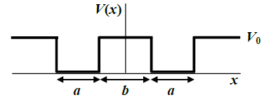
15.5 Kronig-Penney Model:
Inside Wells:,
Outside Wells:,
Impose Bloch Condition on:
We also require the usual continuity of.
These conditions lead to the following equation:
To simplify, we let, while (-function barriers)
with as a measure of the barrier (or scattering strength)
Note that.
For what values of (and) is?
- Plot versus .
- Solutions exist when the function is between -1 and 1 (first figure).
- Plot versus. (There will be two values of that give the same.)
(Go to figures.)
15.6 Reduced Zone Scheme:
- Lattice is periodic-space is periodic
- versus diagram can be reduced to 1st Brillouin Zone from to.
15.7 More Generally:
- versus: Dispersion depends on direction in the crystal.
- Potential is more complex, especially for compounds.
15.8 Feynman Model:
Interactions between atoms lead to energy level splittings:
- 2 atoms: 2 degenerate levelsbonding/ anti-bonding states, 2 levels
- atoms: energy levels (per original level)
(See Figure).
15.8.1 Consider 1-D Array:
Assume only nearest neighbor coupling:
: coupling coefficient
energy in absense of coupling
As before, attempt solution of the form:
Assume that is a function of , since
Try solution of the form
Divide both sides by to get:
This is an allowed energy band.
Larger AWider Band
Similarly, we expect
The generation and analysis of vs. is rather straightforward.(Physical Interpretation)
15.8.2 In 3-D:
Try
16 Implications of Band Theory
- Periodic potential modifies parabolic vs..
Diagram of Free Electron
- Consider motion analagous to that of free electron.
Classically, in electric field,.
In anfield,
Quantum mechanically, we consider electron as wave packet with as.
In a semi-classical picture, then:
But what is?
But
(Alternatively, and .)
So
Rewriting,
But we stated that, implying that electron moves as if it had a mass.
Define effective mass:
Check for free electron:
,
How does this result compare with the Free Electron Model?
To provide a qualitative answer, consider the Feynman Model:
Notes:
- depends on
- Negative around top of band where
- At,
- More overlap Wider bands, smaller
Current Flow for Electrons in a Crystal:
Free Electrons:
Not all electrons in crystal can be accelerated.
From homework,, for particle in box, so for QM electrons:
for since for
But
(Those electrons that can be anticipated.)
Observations:
- is largest when is in the middle of the band (Half-filled).
maximized, high conductivity
- asBand Gap (Filled Band)
, Conductivity (at)
- Number of Electrons per atom will influence the filling of bands, and therfore the type of material.
For Chain of atoms with P.B.C. (Periodic Boundary Conditions):
We need to consider
use Feynman Model to develop understanding
Feynman Model in 2-D
- Bandgaps occur at,.
Example: Choose,,,
- Observe bands“along”:
- Observe bands“along”:
|
|
Conduction
|
|
0.15
|
Electrons, Band #1
|
|
1.0
|
Holes along, Electrons along
|
|
1.5
|
Electrons in Band #2, Holes in Band #1
|
For a single, free electron.
For nearly free electrons in a solid, where .
For a full band: .
If certain electron is missing at top of band:
Note:
So But around top
Remaining electrons act collectively as particle with positive charge.
“Holes” move in opposite direction with opposite charge and therefore make same contribution to current as the electrons.
- Can haveboth, e.g., semi-metals
At finite temperatures, occupation changes according to F-D Distribution, which broadens.
Materials with narrow gaps can become conducting semiconductors.
(Figure #1, Lecture 13)
17 Semiconductors
Classes of Band Structures: (see slides) [1]
- Metals: within one band
- Semi-Metal: within two overlapping bands
- Insulators: within large gap ()
- Semiconductors: within small gap
SemiConductor Sub-Classes: Direct or Indirect Gap [2]
(See Examples of GaAs, AlAs)
Maxima and minima depend on both structure and composition [3]
Energies of Electrons
Electrons move as free particles with effective mass; near band bottom; taking and for reference.
Negative, + charge Positive, - charge
Intrinsic Semiconductors
At finite, electrons occupy conduction band, leaving holes in the valence band.
= density of free electrons
= density of free holes
= intrinisic carrier concentration
conduction band
valence band
From Lecture #9, the D.O.S. (density of states) for free electrons:
For bottom of conduction and top of valence band:
These states become occupied according to:
For in gap and
(Maxwell-Boltzmann)
Examine product graphically to inform the integration:
- is zero in gap.
- is zero at top of band only bottom will matter.
Hence,
Let
, where
Need expression for:
Let
Fermi level is approximately mid-gap for intrinsic semiconductors.
At given temperature, smaller gap implies more carriers and a higher intrinsic carrier concentration.
Extrinsic Semiconductors
Impurities (dopants) added to control
“n -type”: negative charge carriers
- Add atom with extra valence electron: donor
- e.g.,, (Group Ⅴ) to, (Ⅳ).
Donor Level Energy (estimate)
Electron + ionized donor is like atom but in material with
Estimate for Si:
Donor Binding Energy
around
( around)
Most donors are ionized (for)
We showed that
In thermal equilibrium, for, but not too large:
By rewriting in terms of,, one can show, however, that:
can increase the number of electrons, but there will be fewer holes.
(Figure 3-16)
Law of Mass Action
“p-type”: positive charge carriers
- Add atom with 1 less valence electron: acceptor
- e.g. Add,, (Group Ⅲ) to, (Group Ⅳ)
- for at room temperature
Observations
- At very low temperatures, not all donors will be ionized. (Ionization Regime)
- At very high temperatures, becomes appreciable due to thermal activation across gap. (Ionization Regime)
- More generally, both donors and acceptors may be present.The number of free carriers is given by:
- Space-charge neutrality: (in equilibrium)
- Law of Mass Action:
At room temperatures,,
If, e.g.,, then
Compensation: We have a reduced net electron concentration.
18 Current Flow in Semiconductors
(S+W, Chapter 8 and A+M, Chapter 1)
Equilibrium
- Carriers move quickly , but nonet motion of charge.
- Random scattering from phonons and impurities: this randomizes momentum.
- : mean free path between collisions
- average time between collisions (inverse rate)
In Applied Field
Electron feels a force , accelerates, but collisions randomize.
For an average collision, .
In steady state,
where Drift Velocity
where Drift Velocity
, so we have Ohm's Law
, where is the conductivity.
(Note that is a tensor.)
Also, note that (simple interpretation).
for electrons.
Overall, the current due to drift is:
when.
You may be more familiar with , where .
- refers to length; refers to the cross-sectional area
Observations:
Conductivity is proportional to, inversely proportional to.
What are the origins of scattering?
Scattering Mechanisms
- Phonons (Lattice Scattering)
- Impurities/ Defects
(less time near)
- Charge Carriers
(can neglect for moderately doped semiconductors)
Scattering Rate:
Observations:
- Doping increases by increasing,, but impurity scattering also increases.
- At high fields, additional scattering mechanisms lead to non-linear changes in with.
- Si, Ge, velocity saturation (Optical Phonon Scattering)
- GaAs NDR for (Inter-valley Scattering)
Hall Effect
(skipped in 2012)
Experiment used to determine,,,.
for holes.
Assume.
Holes are deflected in direction until field builds up to oppose the flow.

in steady state (
Hall Effect)
(The Hall voltage is)
Note:
Also:
We can therefore determine the majority carrier type and mobility.
Additional Transport Processes: Diffusion
A gradient in free carrier concentration leads to diffusion. (See figure)
Fick's First Law: (1-D)
- refers to flux
- is the diffusion coefficient
- refers to the concentration
These are the diffusion currents:
In the presence of and :
Whereas majority carriers dominate current flow due to drift ( or), minority carrier diffusion currents can be substantial (,).
Consider energy band diagram in presence of applied field. (See att version.)
The energy of an electron is and
So
Electrons drift“downhill.”
Holes drift“uphill.”
Variations inconcentration also reduce fields. Consider holes:
No current when

{Q: What
would produce this? See homework.}
Note that refers to and is zero in the above equation.
Einstein Relation (also holds for electrons)
Concentration Gradients“Built-in” Fields
Inside a semiconductor,
Slope in bands indicates field
Fields result from:
- Applied voltage:
- Carrier concentration gradients
Consider holes in the absense of current:
We can relate drift to diffusion:
Note: and
Substituting above,
So Einsteen Relation (also for)
This assumes equilibrium.
HW Problem #8.4
(in class, 2010, 2011)
- Consider donor doping profile:
- What is the field?
In equilibrium, and
Use Einstein Relation.
Field depends on termperature and rate of dopant decrease (juction abruptness).
-
Additional Homework Solutions:
- Parts (a) and (b):
-
-
Also: (Connects A with B)
( is an estimate)
-
For,
For high fields,
;
is approximate; should be looked up
-
,,
19 351-1 Problems
- Newton’s Laws Can be derived from Hamilton’s equations.
- Identify the Hamiltonian from conservation of energy using only momentum (for Kinetic Energy) and position (for potential Energy):
Use the Hamiltonian for a particle in a 1-D quadratic potential like a mass on a spring. What is ?
- Hamiltion's equations are
Show these give Newton’s laws of motion for the mass on a spring.
- Derive the 1-D differential equation of motion from Hamilton equation. For a particle of total energy E and spring constant , at , what is the equation of motion. what is . show the region of Phase Space ( vs) that describes the particle throughout its motion.
- Use the equipartition theorem (where <A> is time average of A, and is index for each spatial dimension):
to derive the relationship between thermal velocity and temperature
- Derive the Dulong-Petit law for atoms in a 3-D potential from the equipartition theorem:
- What is the heat capacity in this case?
- Problem 1.1 from Solymar and Walsh:
A 10 mm cube of germanium passes a current of 6.4 mA when 10 mV is applied between two of its parallel faces. Calculate the resistivity of the sample. Assuming that the charge carriers are electrons that have a mobility of 0.39 , calculate the density of carriers. What is their collision time if the electron's effective mass in germanium is 0.12 where is the free electron mass?
- Give a one line description of each of these experiments and their significance to modern physics: Photoelectric Effect, Compton Effect, Black Body Radiation, Rutherford Backscattering (Bohr model), Electron Diffraction, Atomic spectra.
Classical: https://www.youtube.com/watch?v=yXsHflXB7QM
Bohr Atom: https://www.youtube.com/watch?v=ydPzEZTd-98
Wave Particle Duality - photoelectric effect: https://www.youtube.com/watch?v=frNLtEm1glg
Schrödinger waves: https://www.youtube.com/watch?v=C8XGIYz1PCw
Probability interpretation: https://www.youtube.com/watch?v=p7xIKoBdViY
Compton Effect: https://www.youtube.com/watch?v=0Y648TNGAIo
- Problem 2.1 from Solymar and Walsh.
Find the de Broglie wavelength of the following particles, ignoring relativistic effects:
(i) an electron in a semiconductor having average thermal velocity at and an effective mass of ,
(ii) a helium atom having thermal energy at
(iii) an α particle ( nucleus) of kinetic energy 10 MeV.
Hint: See question 1. For a gas of non-interacting particles, .
- A particle of mass, , is confined to a 1-D region . In class, we derived the following stationary state wavefunctions and energies for this 1-D infinite square well potential:
- Normalize the wave function to find the value of .
- Find the Energy of these stationary states
Assuming that the initial normalized wavefunction of this particle at is:
- Derive an expression for the wavefunction , at all later times
- Show that the probability of finding the particle in the left half of the box (i.e., in the region ) at time is:
- Assuming that Ψ(x,t) is a solution of the 1-D Schrödinger Equation, the current density is defined as:
In this problem, consider the potential barrier of height () and width () that is depicted in Fig. 3.3 of Solymar and Walsh. Assume that the electron energy () is less than .
- By applying suitable boundary conditions and your knowledge of quantum mechanics, develop a system of equations that could be solved to determine the transmitted current through the barrier () in terms of the incident current on the barrier ().
- By solving your system of equations from part (a), show that:
where and
- In the limit where show that:
- The exponential dependence of the “tunneling” current on distance is utilized for atomic resolution imaging of conductive surfaces with the scanning tunneling microscope (STM). Conservatively assume that the STM can detect changes in the tunneling current of 1%. Under typical tunneling conditions (e.g., , d ~ 10 Å), estimate the vertical spatial resolution of the STM. Hint: The answer can be expressed in picometers ( m)!
- Derive the solution of the 2-D particle in a box (particle is constrained in both , and directions; at the boundaries).
- Solve for the energies and wave functions of the ground and first excited states.
- What is the degeneracy of the first excited state?
- Plot the probability distributions 2 ψ of the first excited states as surface plots.
- Optional: plot probability distributions of the ground state, first excited states, and 2nd excited states, and comment on the evolution.
- Consider the infinite spherical well: if , if .
- For , determine the allowed energies .
- For , show that the corresponding wavefunctions are:
In class, we worked through the Schrödinger equation in spherical coordinates for spherically symmetric potentials by breaking the solution into radial and angular functions. You should be able to solve the radial equation for the conditions given here.
- Consider the infinite spherical well: if , if .
- For , show that there is no bound state if: . This can be shown without resorting to numerical computation.
- Given , find the energies of the two bound states by graphing in MATLAB or Excel. You can also use MATLAB to check your solution by solving the transcendental equation directly.
This problem is analogous to the finite square well problem solved in 3.8 of Solymar and Walsh, but in the spherical coordinate system. Through the appropriate application of boundary conditions, you should arrive at a transcendental equation whose argument can be analyzed to establish the condition for the existence of bound states.
- Suppose that the nucleus of a hydrogen atom is located at a distance d from a two-dimensional infinite potential wall which, of course, tends to distort the hydrogen atom. As approaches zero, determine the following items:
- The ground state wavefunction.
- The degeneracy of the first excited state (ignore degeneracy due to spin).
- The wavelength of light that is emitted upon transition between the first excited state and the ground state (express your answer in nanometers).
With the exception of part (c), this problem does not involve mathematical calculation. The proper choice of coordinate system can make the relationship between these solutions and the usual hydrogen atom solutions clear. Bear in mind that the ground state refers to the lowest energy state that exists.
- Consider a double finite potential well in one dimension. Suppose that the depth and the width are fixed such that the following equation is obeyed:
- Qualitatively sketch the ground state wavefunction and the first excited state wavefunction for: (i) 0, (ii) , and (iii) .
- For , show that the ground state energy ) is given by: , where is the solution of the following equation: . Calculate in units of .
- For, show that the first excited state energy is given by: where is the solution of the following equation: . Calculate in units of .
- For , estimate and in units of .
- Use the MATLAB code derived from Garcia, R., Zozulya, A. & Stickney, J. MATLAB codes for teaching quantum physics: Part 1. arXiv physics.ed-ph, (2007). http://arxiv.org/pdf/0704.1622.pdf
Consult the original publication for background on the code, which is reproduced below.
- What is the Heaviside function? How is it used in this code (for what purpose)?
- Using the MATLAB code, generate the plots you sketched in part (a) (ground and first excited states for b=0, b=a/2, and b>>a). You should have three graphs with two curves on each. Label the graphs and the wave functions.
- Generate 2 more plots with intermediate barrier widths, and sketch the trends in and as a function of barrier width (you should have 5 different widths).
Note: in the code, you can change the potential profile quite easily (e.g. the quadratic harmonic oscillator potential or single square well). Parameters can be varied to develop insight into how the wavefunctions vary with the potentials.
- Provide a physical explanation for the variation of with b that you observed in part (e).
- The double well is a primitive one dimensional model for the potential experienced by an electron in a diatomic molecule (the two wells represent the attractive force of the nuclei). If the nuclei are free to move, they will adopt the configuration of minimum energy. In view of your conclusions in (b), does the electron in the ground state () tend to draw the nuclei together or push them apart? What about ? Provide a physical reason for these behaviors, considering your answer to the previous question.
% Program 4: Find several lowest eigenmodes V(x) and
% eigenenergies E of 1D Schrodinger equation
% -1/2*hbar^2/m(d2/dx2)V(x) + U(x)V(x) = EV(x)
% for arbitrary potentials U(x)
% Parameters for solving problem in the interval -L < x < L
% PARAMETERS:
L = 5;% Interval Length
N = 1000; % No of points
x = linspace(-L,L,N)';% Coordinate vector
dx = x(2) -x(1); % Coordinate step
% POTENTIAL, choose one or make your own
U = 1/2*100*x.^(2); % quadratic harmonic oscillator potential
%U = 1/2*x.^(4); % quartic potential
% Finite square well of width 2w and depth given
%w = L/50;
%U = -500*(heaviside(x+w)-heaviside(x-w));
% Two finite square wells of width 2w and distance 2a apart
%w = L/50; a=3*w;
%U = -200*(heaviside(x+w-a) -heaviside(x-w-a) ...
% + heaviside(x+w+a) -heaviside(x-w+a));
% Three-point finite-difference representation of Laplacian
% using sparse matrices, where you save memory by only
% storing non-zero matrix elements
e = ones(N,1); Lap = spdiags([e -2*e e],[-1 0 1],N,N)/dx^2;
% Total Hamiltonian hbar = 1; m = 1;
% constants for Hamiltonian H = -1/2*(hbar^2/m)*Lap + spdiags(U,0,N,N);
% Find lowest nmodes eigenvectors and eigenvalues of sparse matrix
nmodes = 3; options.disp = 0;
[V,E] = eigs(H,nmodes,'sa',options);% find eigs
[E,ind] = sort(diag(E));% convert E to vector and sort low to high
V = V(:,ind); % rearrange corresponding eigenvectors
% Generate plot of lowest energy eigenvectors V(x) and U(x)
Usc = U*max(abs(V(:)))/max(abs(U)); % rescale U for plotting
plot(x,V,x,Usc,'-k'); % plot V(x) and rescaled U(x)
% Add legend showing Energy of plotted V(x)
lgnd_str = [repmat('E = ',nmodes,1),num2str(E)];
legend(lgnd_str) % place lengend string on plot - Consider a cesium chloride crystal where the potential energy per formula unit is:
where is a constant, , is interionic distance, and is the Madelung constant.
- Express the binding energy () in terms of , and fundamental constants. Hint: first express A in terms of these constants by considering the equilibrium condition.
- The cesium chloride crystal structure consists of cations located on a simple cubic lattice (lattice constant = ) with an anion located at the center of the cube. What is the volume per formula unit () in terms of ?
- From thermodynamics, the bulk modulus (B) is known to be: Show that is of the form , and find . Hint: use your result from the previous problem to rewrite the derivatives in terms of r.
- Using the result from part (c), express the equilibrium bulk modulus () in terms of , and fundamental constants.
- The experimentally determined values of and for CsCl are 19.8 GPa and 3.571 Å respectively. Calculate for CsCl in eV. Note: M = 1.7627 for CsCl.
Nomenclature
- $\epsilon_{0}$
- Permittivity of Free Space ($8.854\times 10^{12} \mathrm{C}^{2}/\mathrm{Jm})$
- $\sigma$
- Stefan's Constant ($5.67\times10^{-8}\mathrm{\frac{W}{m^{2}k^{4}}}$)\\
- $c$
- Speed of Light ($2.998\times 10^{8} \mathrm{m/s}$)
- $e$
- Electron Charge $(1.6022\times10^{-19}$ C)
- $h$
- Planck's Constant ($6.626\times 10^{-34} \mathrm{Js}$)
- $m_e$
- electron mass
- $m_{e}$
- Mass of an Electron ($9.109\times10^{-31}\mathrm{kg}$)\\
Index
- Bohr radius: 1
- electron mass: 1
- Larmor Formula: 1
- Planck's constant: 1