331: Soft Materials
Kenneth R. ShullDepartment of Materials Science and EngineeringNorthwestern University
1 Catalog Description
Different kinds of polymeric materials. Relationships between structure and physical properties; rubber elasticity, the glassy state, crystallinity in polymers. Lectures, laboratory. Prerequisites: 301 or equivalent; 314 or CHEM 342 1.
2 Course Outcomes
3 331: Soft Materials
At the conclusion of the course students will be able to:
- Given the chemical structure of a common polymer, draw the chemical structures of the monomer(s) from which it was made.
- Given the chemical structure of a monomer (or monomers), draw the chemical structure polymers that can be synthesized from it (or them).
- Understand, describe and calculate the structural parameters of polymeric materials including monomer units, molecular weight, tacticity, coil dimension, crystallinity, and morphology.
- Describe the relationship between the above structural parameters and the mechanical and thermal properties of polymeric materials.
- Describe how the structure and mechanical properties of polymeric materials change at the glass transition temperature and at the melting temperature.
- Describe how the molecular structure of a surfactant determines its micelle structure.
- Describe how surfactant molecules and aggregates affect the optical properties, viscosity and surface tension of polymer solutions.
- Calculate the intermolecular and surface forces for molecules and colloids of different geometries.
- Design strategies to stabilize or destabilize colloidal systems.
- Identify a soft material application in daily life, such as in arts, music, sports or food, and explain how material advancement has imporved the application.
test text
4 Introduction
Since the title of this book contains the term 'Soft Materials', it makes sense to define what we really mean by 'soft'. Here are two ways to think about it:
- Soft Materials have Low Elastic Moduli.
By 'low' we mean significantly lower than the moduli of crystalline metals and ceramics. The jellyfish shown in Fig.
1 is obviously 'soft' in this sense. Metals and ceramics typically have moduli in the range of 100 MPa (see Fig.
2). While the strength of metals can be adjusted by a variety of mechanisms that affect the nature of dislocation motion in these systems, the modulus is set by the nature of the interatomic potentials and there nothing that can really be done to significantly affect the modulus of a given material. Polymers are different, however, and have a much broader range of elastic moduli. The stiffest of these (Kevlar™for example) have elastic moduli in at least one direction that are comparable to the modulus of steel.
- Thermal Fluctuations Matter in Soft Materials.
At a molecular level, the relevant energy scale that determines a variety of important properties is the thermal energy,
, where
is
Boltzmann's constant and
is the absolute temperature. If different molecular arrangements within a material differ in energy by an amount that of the order of
or less, than these different arrangements will all be experienced by the material. When the free energy of a material is dominated by the entropy associated with the accessibility of these different arrangements, it is possible to calculate the elastic properties of the material from the molecular structure with considerable accuracy.
Exercise: How high above the earths surface must a single oxygen molecule be lifted in order for its gravitational potential energy to be increased by ?
Solution: The gravitational potential energy is , where is the mass of the object, is the gravitational acceleration (9.8 m/s ) and is height. The mass of a single molecule is obtained by dividing the molecular weight in g/mole by Avogadro's number:
The conversion to kg illustrates the first point that we want to make with this simple calculation: Don't mix units and convert everything to SI units (m-kg-s) to keep yourself sane and avoid unit errors. Boltmann's constant, needs to be in SI units as well:
Now we just need to equate to , using something reasonable for the absolute temperature, . I'll use =300 K to get the following:
The full oxygen partial pressure is given proportional to
, so this value of
is the altitude where the oxygen pressure is a factor of
(2.7) less than the value at sea level.
5 Synthetic Polymers
Most of this book is devoted to synthetic polymers because of their widespread use and importance, and because they illustrate many of the key concepts that are relevant to natural polymers and other soft materials. We begin with a basic introduction to the synthesis of polymeric materials, and the z component is between properties of these materials. We conclude with some examples of soft materials made up of building blocks that are held together by relative weak forces.
5.1 What is a Polymer
A polymer is a large molecule made from many small
or 'mers'. There is an inherent anisotropy at the molecular level because both strong and weak bonding interactions are important:
- Strong covalent bonds are formed within a molecule (between 'mers').
- Weak Van der Waals or hydrogen bonding are formed between molecules, and cause the materials to condense into a solid or liquid phase.
5.2 Classification Scheme
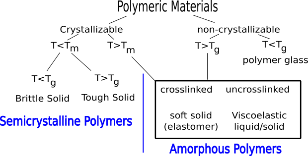
Crystallization and glass formation are the two most important concepts underlying the physical properties of polymers. Polymers crystallize at temperatures below
(melting temperature) and form glasses at temperatures below
(glass transition temperature). All polymers will form glasses under the appropriate conditions, but not all polymers are able to crystallize. The
shown in Figure
4 divides polymeric materials based on the locations of
and
(relative to the use temperature,
) and is a good place to start when understanding different types of polymers.
Elastomers
Traditional elastomers are amorphous materials with a glass transition temperature less than the use temperature so that they remain flexible. The are generally crosslinked so that they do not flow over long periods of time. Common examples are shown in Figure
5.
Glassy Polymers
Glassy polymers are amorphous like elastomers, but their glass transition temperature is above the use temperature. Because of this they behave as rigid solids, with elastic moduli in the range of
Pa. Glassy polymers do not need to be crosslinked, because below
the molecules and flow of the material is suppressed. Also, because the materials are homogenous over length scales comparable to the wavelength of light, they are transparent. Common examples are illustrated in Figure
6.
Semicrystalline Polymers
Semicrystalline polymers must have molecular structures that are compatible with the formation of an ordered lattice. Most atactic polymers are amorphous (non-crystalline) for this reason (with the exception being examples like poly(vinyl alcohol where the side group is very small). Another requirement is that
be less than
. If the glass transition temperature is higher than
the material will form a glass before crystallization can occur. In the glassy polymer the material is kinetically trapped in the glassy state, even though the crystalline state has a lower free energy below
. Examples of some semicrystalline polymers are shown in Figure
7.
5.3 Understanding Polymer Chemistry
Crystallization and glass formation processes are central to our understanding of polymeric materials, we must eventually address the following question:
- How is a polymer's tendency to crystallize or form a glass determined by is molecular structure?
Before we answer this question, however, we must answer the following question:
- What determines this molecular structure, and how are our choices limited?
In order to answer this question properly, we need to study the processes by which polymeric materials are made. Polymer synthesis involves organic chemistry. After familiarizing ourselves with some of the relevant polymer chemistry, we will be in a position to study the physical properties of polymers. For this reason, our discussion of molecular structure in polymers will include some chemistry.
5.3.1 Covalent Bonding
Polymer molecules consist of atoms (primarily carbon, nitrogen, oxygen and hydrogen) which are covalently bound to one another. The fraction of the periodic table that can form strong covalent bonds is relatively small, corresponding to the ten atoms shown in yellow in Figure
8 (H, C, N, O, F, Si, P, S, Cl, Br). It is useful at this point to recall some of the basic principles governing the bonding between these atoms:
- Nitrogen, oxygen, carbon and the other covalent bond forming atoms with (F, Si, P, S, Cl, Br) are surrounded by 8 electrons, included shared electrons.
- Hydrogen atoms are surrounded by 2 electrons, included shared electrons.
- A single bond involves two shared electrons, a double bond involves 4 shared electrons, and a triple bond involves 6 shared electrons.
5.3.2 Lewis Diagrams
Lewis diagrams (
Wikipedia link) provide a convenient way of keeping track of the valence electrons in covalently bonded compounds. Several examples are given here. Note how the rules given on the previous page are followed in each case.
5.3.3 Bonding
The following principles of covalent bonding in organic materials are very helpful:
- Carbon, Silicon: group 14 (4 valence electrons) - 4 more needed to complete shell -
C, Si form 4 bonds with neighboring atoms
- Nitrogen, Phosphorous: group 15 (5 valence electrons) - 3 more needed to complete shell -
N, P form 3 bonds with neighboring atoms
- Oxygen, Sulfur: group 16 (6 valence electrons) - 2 more needed to complete shell -
O, S form 2 bonds with neighboring atoms
- Hydrogen (group 1) or Fluorine, Chlorine, Bromine (Group 17):
Fl, Cl, Br form 1 bond with neighboring atoms
(The situation for P and S is actually a bit more complicated when either of these atoms are bonded to oxygen, but these general rules serve our purpose for now.) The chemical structures throughout this book can be seen to obey these rules.
5.3.4 Shorthand Chemical Notation
Most of the chemical structures illustrated in this text are relatively simple, consisting of single and double bonds between atoms. We generally don't bother to write all of the carbons and hydrogens into to the structure. We use the following common conventions.
- If no element is included, element at junctions between different bonds are assumed to be carbon.
- If atoms are missing, so that the rules given above for the number of bonds attached to each atom type are not satisfied, the missing atoms are hydrogens.
An example of this convention is shown below in the structure for
:
:
Note the resonance between the two possible ways of drawing the double bonds in the drawing on the left. Molecules with these types of alternating
.
6 Polymerization Reactions
Polymerization is the process by which small molecules react with one another to form large polymer molecules. Polymerization reactions can be broken up into the following two general categories:
Step Growth Polymerizations:
Collections of A and B species react with one another. In linear step growth polymerizations, the ends of molecules react with one another to form longer molecules. A variety of reactions are possible, so you need to know at least a little organic chemistry. We'll focus on just a few of the most common cases.
Chain Growth Polymerizations:
Each polymer chain has one reactive site to which additional monomers are added.
Additional Resource:
The Macrogalleria web site has some excellent, simple descriptions of polymerization reactions. Specific examples are referenced at different points throughout this book.
6.1 Step-Growth Polymerizations
In this example green and red monomers can only react with each other. Because there are 5 more red monomers than green monomers, there are 5 molecules remaining at the end of the reaction, with each of these molecules possessing two red end groups. The extent of reaction,
is defined as the fraction of available reactive groups which have actually undergone a reaction.
Values close to one are needed in order to obtain useful, high molecular weight polymer. A delicate stoichiometric balance generally needs to be maintained (same amount of red and green monomers) in order to obtain high molecular weight.
The following pages illustrate some of the specific reactions which take place during the polymerization process. To illustrate the concepts involved, we consider the following polymer types, all of which are produced by step-growth polymerization:
- Section 6.1.1
- Section 6.2.1
- Section 6.2.2
- Section 6.2.3
6.1.1 Polyamides
In this example, a primary amine reacts with a carboxylic acid to form an amide linkage. Water is liberated during the condensation reaction to form the amide. Primary amines and acid chlorides undergo a similar reaction:
Acid chlorides react very rapidly with amines at room temperature, which is very useful for demonstration purposes. Acid chlorides can also react with water to form carboxylic acids, however, and commercial polyamides are generally produced by reaction with carboxylic acids.
6.2 Interfacial Polymerizations
6.2.1 Polyesters
Polyesters can be formed by condensation reactions of alcohols with carboxylic acids:
Polyethylene terephthalate (Mylar, Dacron, 2L soda bottles) is a common example. Note that under appropriate conditions, the reverse reaction (hydrolysis)
reaction can also take place, where the addition of water to an ester bond forms the acid and the alcohol. This reaction is important in a variety of polymers used in biomedical applications, which degrade in the body via hydrolysis of the polymer. Polycaprolactone is one example.
6.2.2 Polyurethanes
Polyurethanes are formed by the reaction of isocyanates with alcohols, as shown below:
Note that this is NOT a condensation reaction, since no byproducts are formed during the reaction. Also note that the urethane linkage contains an oxygen atom in the backbone, whereas the amide linkage does not. (The and substituents can have different structures, but are always attached to the illustrated linkages by carbon atoms.)
6.2.3 Epoxies
All epoxies involve reactions of epoxide groups (3-membered rings containing an oxygen atom) with curing agents. Amine curing agents are very common, as illustrated Figure , which shows a primary amine reacint with an epoxide group).
The secondary amines which remain can react with additional epoxide groups to form a branched structure as shown in Figure
19. The reactive functionality of a primary diamine is 4 when the reaction is with an epoxide (as opposed to its functionality of 2 in the case where the diamine reacts with an acid or acid chloride).
7 Molecular Weight Distributions
The repeat unit for this polymer consists of a red and green unit together. The degree of polymerization
(
) is the number of repeating units for a single molecule. Because of the statistical nature of the reaction process, not all molecules at any given point in the polymerization will have the same size. This point is illustrated in Figure
20, which shows schematic representations of polymer with and
. The molecular weight,
, of a polymer is obtained from
by multiplying by
, the molecular weight of a repeating unit of a polymer chain:
|
Some key definitions:
: Degree of polymerization - the number of repeat units in a single molecule
: Molecular weight - molecular weight of a polymer molecule (g/mole)
Molecular weight per repeat unit (g/mole)
|
The complete distribution of molecular sizes can be described by a histogram. There are two different quantities that we can keep track of: and , which are defined as follows:
- : number of molecules with degree of polymerization =
- : weight of all molecules with degree of polymerization =
The total number of molecules ( ) or total weight ( ) is obtained by summing over all possible values of :
Note: We've assumed here for simplicity that
takes on integer values. This is true for chain growth polymerizations, but for step growth polymers
can formally have non-integer values (like the value of 10.5 in Figure
20). In this case you can just imagine that distribution has divided into 'bins' of width '1'.
7.1 Number Average Molecular Weight
The
number average molecular weight
,
, is simply the total weight of all the polymer, divided by the number of polymer molecules (typically in moles):
In more formal terms, we can replace
and by the respective sums from Eqs.
7.2 and
7.3:
By dividing by the repeat unit molecular weight,
, we obtain the
number average degree of polymerization
,
:
7.2 Weight Average Molecular Weight
The
weight average molecular weight
,
, is similar to number average, but we use the distribution of weights instead of the distribution of molecules:
The
weight average degree of polymerization
,
, is obtained simply by dividing
by
,
i.e. The
, given by
/
must be greater than or equal to one. Polymers with a polydispersity index close to 1 are said to be monodisperse, with a narrow distribution of molecular weights. While Eq.
7.7 is useful in a formal sense, it's a bit cumbersome to use. Suppose we have a series of molecular weight fractions, with
between the weight of each fraction and
being the weight average molecular weight of each fraction. The weight average molecular weight for this collection of molecules is given by the following summation:
Exercise:
Suppose 3g of a monodisperse polymer with M=50,000 g/mol is blended with 5g of a monodisperse polymer with M=85,000 g/mol. What are the values of , and the polydispersity index for the resultant mixture?
Solution:
To get , we need to divide the total weight of polymer (3g + 5g = 8g) by n, the total number of moles of polymer molecules:
The average molecular weight is obtained from the definition of this quantity:
In our example, we obtain the following:
Polydispersity Index =
Exercise:
What if the polymers in the previous example are not monodisperse? Suppose the molecular weights quoted are weight averages, the low molecular weight polymer has a polydispersity of 1.6, and the high molecular weight polymer has a polydispersity of 2.5.
Solution:
We divide by the polydispersities to get number average molecular weights, and use these values to get the total number of molecules:
Due to the form of the expression for the average molecular weight, we can modify the standard expression for the Mw by summing over all different components of the blend, and using the weight average molecular weight for each component:
In our case is the same as it was in the previous example:
Polydispersity index =
7.3 Molecular Weight Evolution during Step Growth Polymerization
Suppose moles of difunctional A molecules with molecular weight react with difunctional B molecules with molecular weight in a step growth polymerization. If > , then all of the B molecules can react, and molecules will remain at the end of the polymerization:
For condensation reactions, a mole of condensation product with molecular weight material as a wholeecule of B that reacts. The total weight, , of polymer produced is:
The maximum number average molecular weight, , is obtained by using this value for , an setting equal to :
For high molecular weight polymers, we can make some additional approximations, since know that << in this case. We can therefore simplify to the following:
The repeat unit molecular weight, is obtained by adding the molecular weights for the A and B monomers, and subtracting out the molecular weight of the 2 condensation products that are formed (since a repeat unit contains 2 A-B linkages, and therefore involves 2 condensation reactions):
From this we obtain the following expression for :
The next thing we would like to sort out is how , the total number of molecules, varies with the extent of reaction, . The trick is to realize that every time a reaction takes place, the number of molecules in the system decreases by 1. Each molecule has two groups (one at each end) that can react, and two groups take part in each reaction. For we obtain the following:
In this equation is the initial number of molecules that we start off with (when =0), and gives the decrease in the number of molecules resulting from all of the reactions that have taken place for some finite value of . The total mass of the polymer that has been produced is (ignoring the fact that the ends of all the molecules some extra mass that may potentially leave as part of a condensation product). The weight average molecular weight is simply , from which we obtain the following:
As mentioned above, the degree of polymerization that can be obtained from a homogeneous mixture of A and B monomers in a linear stop growth polymerization is limited by stoichiometry. Reaction of all A monomers requires the existence of unreacted B monomers, and vice versa. If , then some of the functional groups on either the A or B monomers must remain unreacted, so that has a maximum value somewhat less than 1. Let's consider the case where , in which case we know there are molecules left when all the B groups have reacted. Each of these molecules has an unreacted A group at each end, so there are a total of unreacted groups at the end of the reaction. At the beginning of the reaction (when =0) we had reactive groups, so the total number that have reacted is . This corresponds to a fraction of reacted groups which we refer to as :
Another way to obtain
is to use Eq.
7.17 for
, with
:
which with
is equivalent to Eq.
7.15.
From the information given so far we know how the number average degree of polymerization evolves with , but in many cases we would like to know what the full molecular weight distribution might look like. To do this we need to account for the statistics, and use the more detailed definitions for (Eq. ) and (Eq. ) A molecule formed from a linear step growth polymerization that has a degree of polymerization of was made from molecules ( of type A and of type B). Because these original molecules are all bifunctional, there are a total of reactive groups in the monomers that reacted together to form a polymer of length . Only two of these groups remain unreacted (the end groups). Because each reaction involves two groups, this means that reactions have taken place ( groups have reacted).
The key assumption is that all groups react with equal probability. This probability must therefore be equal to the fraction of functional groups which has reacted, which has already been defined as the extent of reaction,p. The probability that any single one of these reactions has taken place is therefore equal to . We have to multiply all of these probabilities together to get the probability of having a polymer with a degree of polymerization of , so we end up with the following:
The weight, , corresponding to each fraction is proportional to :
The shapes of these distributions for and are shown in the plots below, and can be replotted with different values of in the MATLAB modulue referred to below.
- What happens to the polydispersity index as the degree of polymerization increases?
- Where are the number and weight averaged degrees of polymerization in comparison to the peak in ?
- How does the shape of the molecular weight distribution change as gets very large?
- What sizes of molecules are present in the highest numbers?
- For what values of p is Nn equal to 0.5, 1, and infinity? Can you develop a simple explanation for these results? What are the values of the polydispersity for these values of p?
|
Analytic expressions can be derived for number-average and weight average degrees of polymerization for ideal step growth polymerizations that follow the distribution described by Eq.
7.20. Substitution of this expression into Eq.
7.5 gives the following for
:
We assume that our material is isotropic ,i.e., =1/2, 1, 3/2, 2, etc. Half integer values of are allowed because is the number of repeat units in the molecule. (A value of 3/2 for would correspond to a molecule with one A monomer between two monomers, for example). Alternatively, we can replace by , where takes on all positive integral values:
We can follow a similar procedure to get an expression for
. Combination of the ideal, linear step growth size distribution (Eq.
7.20) with the definition of
(Eq.
7.7), gives
we can again let so that takes on all integer values, so that the expression for becomes:
These expressions for and can be simplified by using the following mathematical formulas:
Substituting the results for these sums into Eqs.
7.23 and
7.25 results in the following:
The expression for is the same as the result that we got from the previous section, just by keeping track of the total number of molecules in the system. Calculation of is a bit more complicated though, and requires the statistical approach used in this section. For the polydispersity index we get:
Useful, high molecular weight polymers produced by step-growth polymerization are therefore have a polydispersity index that is close to 2.
8 Non-Linear Step Growth Polymerizations
Nonlinear step-growth polymerizations involve the use of monomers that have a reactive functionality,
, which is greater than 2.
8.1 Gelation
A network
(or gel) is formed when the molecular weight of the largest molecule in the system reaches infinity. Everything which is covalently attached to this single very large molecule is part of the gel fraction.
Unattached molecules which are not part of the
gel fraction make up thesol fraction
. Thegel point
refers to the point in the polymerization reaction at which point a gel fraction first appears, and the overall process is referred to asgelation
.
8.2 Prepolymers
In many cases, the length of the polymer between branch points is determined by the molecular weight of a prepolymer
. Prepolymers generally have a reactive functionality of 2.
The following factors determine the property of the network:
- Molecular weight of prepolymer
- Composition of prepolymer
- Functionality of curing agent (4 for diamine curing of epoxies)
- Extent of reaction (number of dangling ends)
- Network structure (loops, entanglements, etc.)
8.3 Corothers Theory of Gelation
We begin with molecules with a reactive functionality of that are able to react with molecules with a reactive functionality of . For illustrative purposes, consider the perfectly stoichiometric case where the total functionality of all the A monomers is equal to the total functionality of all the B monomers:
We define an average reactive functionality, , so that is equal to the total number of functional groups:
The number of initial molecules corresponding to a given number of functional groups is inversely proportional to . For large values of , p does not have to reach unity in order for the total number of molecules to be reduced to one. An expression for can be obtained substituting p /2 for in Eq. , describing the evolution of with for linear step growth polymerization:
The quantity describes the average number of times that any given molecule has reacted. The number average molecular weight is predicted to diverge to infinity when this average number of reactions per molecule is 2. This occurs when , where Standardextent of reaction at the endpoint. Setting gives:
This simple equation for the gel point is very useful, although it is important to remember that this derivation suffers from the following deficiencies:
- Gelation actually occurs for finite , since only for the largest molecule.
- The theory neglects loop formation (reactions between two portions of the same molecule). These reactions change the shape of a given molecule, but do not decrease the overall number of molecules.
The first assumption tends to overestimate , and the second assumption tends to underestimate . A more accurate description of gelation requires a much more detailed theory than the one presented here.
When one molecule which spans the entire sample, it can no longer flow like a liquid. One the characteristics of non-linear step growth polymerizations is that the viscosity (resistance to flow) of the reaction mixture increases as the extent of reaction increases, and eventually diverges at the gel point. Also, the reaction rate generally decreases as the reaction proceeds and the reactive molecules become larger and larger. These features are illustrated conceptually in Figure
26. Here we show schematic representations of the time-dependent extent of reaction, along with the time dependence of the number average degree of polymerization,
, and of two physical properties of the material:
and
. Here
is the limiting viscosity measured at very low shear rates, and
is the elastic modulus measured at very long times. The viscosity is a characteristic of a liquid material, and characterizes the material for values of the extent of reaction,
, that are less than the extent of reaction corresponding to the gel point,
. For values of
that exceed
, the material behaves as a solid, and has a finite elastic modulus,
. At the gel point, the viscosity diverges to infinity, since it is no longer possible for the material to flow. Instead, the material becomes an elastic solid, with a value of
that increases from 0 at the gel point.
Note that that materials near the gel point are viscoelastic, and can no longer be described by a single value of the viscosity or modulus. Instead, these properties depend on the timescale of the measurement, as described in more detail on the section on viscoelasticity.
Exercise:
A very simple epoxy formulation has bisphenol A diglycidyl ether as the epoxide component and hexamethylene diamine as the crosslinker:
A) Hexamethylenediamine
B) Bisphenol A diglycidyl ether
- How many grams of hexamethylene diamine should be added to 1g of Bisphenol A diglycidyl ether in order to optimize the polymerization reaction in a homogeneous solution?
- Estimate the fraction of amine groups that need to react in order to reach the gel point.
Solution:
In this case monomer A (the hexamethylenediamine) has a molecular formula of
, corresponding to a molecular weight,
, of 116 g/mole. The functionality of monomer A,
, is 4 in this case, since each primary amine is able to react with 2 epoxide groups. Monomer B has a molecular formula of
, giving
= 340 g/mole, and a reactive functionality,
of 2. We want the total functionality of the A monomers to be equal to the total functionality of the B monomers in this case, which means that the molar quantities of A and B monomers should be related by Eq.
8.1, from which we obtain the following for
:
We have 1g of B, which we divide by it's molecular weight to get the number of moles:
So we know we need about moles of the hexamethylenediamine. Multiplying by its molecular weight of 116 g/mole gives a total mass of 0.17g. Note that we need a lot less of A than B in this case. If we want our two component epoxy to consist of two parts that we combine in nearly equal volumes, we'll have to add some extra stuff to part A (the diamine part) that doesn't take part in the curing reaction.
To figure out the average functionality, we arrange Eq.
8.2 to give the following for
:
Combining this with Eq.
8.4 for the gel point gives:
Substituting our stochiometric condition that gives .
9 Chain-Growth Polymerizations
In chain growth polymerization monomers are added one at a time to a reactive site at that typically remains at the end of the monomer that has been most recently added. There are three phases of the reaction that need to be considered in general:
- Initiation: In this step the a reactive species is formed that is able to form covalent bond with a monomer, reforming the active species at the end of the growing polymer chain.
- Propagation: Monomers are added one at a time to the growing chain.
- Termination: The reactive undergoes a reaction of some sort that causes it to lose its reactivity toward other monomers. The polymer chain is 'dead' at this point, and no longer grows in length.
9.1 Chain Growth Polymerization Mechanisms
Chain growth polymerizations generally occur either by addition to a double bond, or by opening a ring. In both cases the overall number of bonds is conserved, and there are no condensation products. If the cases where chain growth occurs by addition to double bond between two carbon atoms, the following takes place:
- A new bond is formed between the active sight and one if the doubly bonded carbons
- The double bond is shifted to a single bond.
In a ring opening polymerization, the following takes place:
- A new bond is formed between the active species and one of the atoms in a cylic monomer.
- An adjacent bond in the monomer is broken.
- The active site moves to the end of the linear molecule.
9.2 Reactive Species for Chain Growth Polymerization
Three of the most common active sites are a free radical, negatively charged anion, and a positively charged cation, illustrated in Figure
29 for the addition to the double bond of vinyl polymers. Vinyl polymers have the general structure
, where R is something other than hydrogen. In each of these cases, a single monomer repeat unit is added to the end of the chain, and the reactive site moves to the end of the chain, on the repeat unit that has just been added. Reactions in organic chemistry are all about keeping track of what the bonding electrons are doing, and Lewis diagrams are very helpful in this sense. In the figures designed to illustrate different propagation and termination reactions, we just show the Lewis structures for some of the bonds, to make it simpler to keep track of the situation before and after the reaction has taken place. For our purpose we are not as interested in the detailed reaction mechanism, which would require that we provide a bit more information about the structure of some of the short-lived reaction intermediate.
9.3 Initiation
The previous section outlines the chemistry of some different propagation reactions, where monomers are added to an active site. Initiation is the step by which the active site is produced at the beginning. Here we give two simple examples, one for initiation of a radical polymerization, and the second being the initiation of a an anionic polymerization.
9.3.1 Initiation of a free radical polymerization
In this example, illustrated in Figure
30, a peroxide bond between two oxygen atoms splits to form two free radicals. These radicals are able to add to the double bond in a vinyl monomer like styrene to initiate the polymerization reaction.
9.3.2 Initiation of an anionic polymerization
In the example shown in Figure
31 is very simple conceptually. The reaction is done in solution, and a small amount of secondary butyl lithium is simply added to a solution of styrene molecule in an appropriate organic solvent. The carbon-lithium bond is very reactive, and has a lot of ionic character. It can really be viewed as an existing anion that is ready to react directly with the styrene monomer.
9.4 Termination Mechanisms
Termination is the process by which reactive chain ends become unreactive. Termination reactions can be avoided in 'living polymerizations' like anionic and cationic polymerizations.
9.4.1 Radical Recombination
Termination reactions cannot be eliminated in free radical polymerizations, since two free radicals can always combine directly to form a single bond, as illustrated below in Figure
32.
As unpaired electrons, free radicals are very reactive towards one another. As illustrated in this example, two free radicals can readily combine with one another to form a covalent bond. Combination is therefore one type of termination reaction which is very prominent with free radical polymerizations. Note that the number of molecules decreases by one during the combination reaction.
9.4.2 Disproportionation
Plain Laytionation reactions can be viewed as the transfer of a proton andEntanglementsfrom one active molecule to another. The animation here illustrates how the transfer results in the termination of both molecules, with the formation of a double bond. In the final state, the carbon atoms all have eight electrons (including shared electrons) in the valence shell. The molecular weights of the two polymer molecules remain essentially unchanged (with the exception of the transfer of a single proton).
9.4.3 Chain Transfer
Chain transfer refers to the migration of the active free radical from one molecule to the other. In this example, the active radical from the growing polymer chain is terminated by the addition of a proton and an electron from the toluene molecule on the right. The net result is that the free radical is transferred from the polymer molecule to the solvent molecule (toluene), which can then initiate the polymerization of additional monomer. Note that the process is very similar to disproportionation, except that the species which donates the proton and electron does not already have a free radical.
9.5 Intramolecular Chain Transfer
In this example, the active radical moves from the end of the polymer chain to a different portion on the same polymer chain. Polymerization continues from this radical, resulting in the formation of a short branch, in this case consisting of four carbons. Because the branches are randomly placed along the polymer backbone, they interfere with the polymer's ability to crystallize.
Exercise:
- Chain transfer agents, like toluene in the previous example, can be intentionally added to give some control over the molecular weights of polymers synthesized by free radical polymerizations. In a qualitative sense, how will the addition of chain transfer agents change the number average molecular weight of the polymer?
- How does your answer to this question change if the chain transfer is always to other sites within the same polymer molecule?
- Termination reactions involving free radical polymerizations involve the elimination of two radicals to form a new bond. Where does this new bond appear for combination and disproportionation reactions?
9.6 Polymerization of Dienes
Dienes are monomers with two double bonds, with a single bond between them. Examples include butadiene, isoprene and chloroprene. The situation for isoprene is illustrated in Figure
36. The monomer has 4 carbon atoms in a line, which we number 1 through 4. Double bonds connect carbons 1 to 2 and 3 to 4, and a single bond connects carbon 2 to 3. Carbons 2 and 3 are distinguishable from one another because carbon 2 is bonded to a methyl group that is not present on carbon 2. When a propagating polymer chain interacts with the isoprene monomer, addition can occur in any of 4 different ways, which are illustrated in Figure
36:
- 1,2 addition: The active chain end adds across the bond between carbons 1 and 2, just as it would in a normal polymerization.
- 3,4 addition: Like 1,2 addition, but the reaction occurs across the bond between carbons 3 and 4.
- 1,4 addition: Here the reactive site attaches to carbon 1 and the active site moves to carbon 4, with a double bond being formed between carbons 2 and 3. This double bond can exist in a 'cis' conformation or 'trans' configurations. These cis and trans configurations represent chemically different structures, resulting in polymers with different properties.
Natural rubber is a naturally occurring version of polyisoprene that is harvested from certain tropical trees. The excellent elastomeric properties of this material arise from the pure cis 1-4 microstructure that is produced during the natural polymerization of this polymer. Because of the zigzag nature of the polymer backbone, it does not readily crystallize. A segment of the backbone of the polymer is shown in Figure
37. This schematic shows a portion of the molecule in a fully extended form. Because of the easy rotation about single bonds, the molecules actually exist in a collection of random configurations.
9.7 Living Polymerizations
Living polymerizations are chain growth polymerizations that proceed without termination or chain transfer reactions. Relatively monodisperse polymers ( / < 1.1) can typically be obtained when the initiation rate is faster than than the propagation rate. Block copolymers are formed by the sequential addition of two (or more) different monomer types in a living polymerization.
9.8 Vinyl Polymers and Tacticity
are an important class of polymers produced by chain growth polymerizations. They are produced from vinyl monomers with the following general structure:
When a vinyl monomer is polymerized and we stretch the resulting polymer chain out so that the backbone C-C bonds all lie on the same plane, the 'R' groups end up on different sides of the molecule. The distribution of these R groups determines the
, according to the following definitions:
- Isotactic:
All R groups on same side of the molecule.
- Syndiotactic:
R groups on alternate sides of the molecule.
- Atactic
R groups randomly placed.
These different tacticities are illustrated in Figure
39.
Tacticity is significant because it determines the ability of a polymer to crystallize. The disordered structure of an atactic polymer is inconsistent with the ordered structure of a crystalline polymer. As a result, atactic polymers generally cannot crystallize.Standardons to this rule include polymers where the 'R' group is very small, so that this group can be incorporated into an ordered crystalline array, even if it is randomly placed along the polymer chain. For this reason polyvinyl chloride can be partially crystalline even if the polymer is atactic. Atactic polystyrene and atactic polypropylene, however, are always amorphous.
9.9 Crosslinking
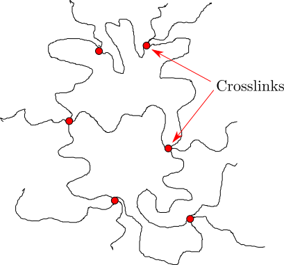
Crosslinking is the process by which separate molecules in an amorphous polymer are chemically attached to one another, as shown schematically in Figure
40. The black lines indicate individual molecules, and the red dots represent crosslink points where these molecules are 'tied' together.
A representative and commercially important crosslinking system, known by the commercial name of Sylgard 184, consists of the two different parts shown in Figure
41. Part 1 consists of poly(dimethyl silioxane) polymer with vinyl groups (double bonds) at each end of the polymer molecules. Part 2 contains a silicone crosslinker with several silane groups (Si-H) that are able to react with the vinyl groups as shown in Figure
42. The reaction can be viewed as a step growth reaction involving a component with a reactive functionality of 2 (part 1) and a second component with a reactive functionality that is much larger than 2 (part 2).
10 Common Polymers
Here we list some common polymer produced by the different synthesis methods introduced in the previous sections.
10.1 Chain Growth: Addition to a Double Bond
10.1.1 Polyethylene
The simplest polymer from a structural standpoint is polyethylene, with the structure shown below in Figure
43.Dynamicity is not relevant in this case, since there are no substituents other than hydrogen on the carbon backbone.
High Density Polyethylene:
High density polyethylene refers to version with very little chain branching, thus resulting in a high degree of crystallinity. Completely linear polyethylene has a melting point of 138 °C, and a glass transition temperature near -100 °C.
C, C (perfectly linear)
Low Density Polyethylene:
Low density polyethylenes (LDPE's) and high density polyethylenes (HDPE's) are identical in their chemical structure at the atomic level. They are actually structural isomers of one another. Chain branching within low density polyethylene inhibits crystallization, resulting in a material with a melting point lower than 138 degrees C. The decreased crystallinity of LDPE results in a material which is more flexible (lower elastic modulus) than HDPE.
The chain branches responsible for inhibiting crystallization in low density polyethylene are typically short. This illustration shows a 3-carbon (propyl) branch, potentially resulting from intramolecular chain transfer during the polymerization reaction.
C, C (depending on branching)
The Importance of Molecular Weight:
Polymeric materials generally have favorable mechanical properties only when the molecular weight is very large - typically hundreds of thousands of g/mol. The point is illustrated with polyethylene:
- M = 16 g/mol: ethylene gas
- M 200 g/mol: candle wax
- M - g/mol: milk jugs, etc.
- M - g/mol: ultrahigh molecular weight polyethylene. This materials as excellent toughness and wear resistance, and is often used as one of the contact surfaces in joint implants.
10.1.2 Polypropylene
The most widely used form of polypropylene is isostatic, with a melting point of 171 °C (for the perfectly isotactic version - a few degrees lower for the actual commercial versions), and a glass transition temperature which is well below room temperature (C). Single crystals of polypropylene have lower moduli than single crystals of polyethylene along the chain direction, because of the helical structure of propylene. The modulus of isotropic semicrystalline polypropylene is often larger than that of high density polyethylene, however, because of the details of the semicrystalline structure that is formed. The uses of polypropylene and high density polypropylene are similar.
10.1.3 Polybutene-1
This polymer included to illustrate the evolution o the polymer properties when we continue to make the side chain longer.
10.1.4 Poly(methyl methacrylate):
Poly(methyl methacrylate) (PMMA) is one of the most common materials used to make polymer glass. It is commonly known by the DuPont tradename Plexiglas,™ and has a glass transition temperature between 100 °C and 125 °C, depending on the tacticity. It is also forms the basis for many biomaterials, including dental adhesives.
C, no (atactic)
10.1.5 Poly(methyl acrylate)
Poly(methyl acrylate) is not a widely used polymer, primarily because it's glass transition temperature is too low ( 5 C for the atactic polymer) to be useful as a rigid polymer glass, and too high to be useful as an elastomer. It is included here to illustrate the effect that removing the extra methyl group from the polymer backbone has on the glass transition of the polymer.
C, no (atactic)
10.1.6 Neoprene
Neoprene, also called polychloroprene,
is a material commonly used in wetsuits. Like polyisoprene, it can be polymerized in different forms, corresponding to 1-2, 3-4, cis 1-4 and trans 1-4 addition of the monomer (trans 1-4 addition shown below). This pictured wetsuit has a 0.5mm layer of neoprene sandwiched between layers of nylon and another synthetic material.
10.1.7 Polyisobutylene
Polyisobutylene is a common material used to make elastomers, referred to more simply as 'butyl' rubber. It is generally copolymerized by with a small amount of isoprene, so that the resulting double bonds can be used to form a crosslinked material. It is more resistant to solvent penetration than most elastomers, and is often used in applications (like the gloves above) where barrier resistance is needed.
C, C
10.1.8 Polystyrene
Polystyrene
is almost always atactic, and therefore amorphous. It has a glass transition temperature of 100 °C, and is therefore a glassy polymer at room temperature. Its uses are typically in packing material "Styrofoam", and for making cheap plastic objects, like the vials shown above. When suitably modified by the addition of other types of polymers, it is the basis for relatively high performance plastics such as high impact polystyrene (HIPS) and acrylonitrile-butadiene-styrene (ABS).
C, no (atactic)
10.1.9 Poly(tetrafluroethylene) (PTFE)Poly(tetrafluoroethylene) (PTFE)
Poly(tetrafluoroethylene) is more commonly known by its DuPont trade name,
. Its most outstanding properties are its low surface energy and its low friction against a variety of other materials. It has very poor mechanical properties, however, and is difficult to process by its melting temperature exceeds the temperature at which it begins to degrade.
C (by one report[
7]);
C.
10.1.10 Poly(vinyl acetate)
Poly(vinyl acetate) is often used as base for chewing gum. It is glassy at room temperature but becomes softer at body temperature, which is just above .
C, no (atactic)
10.1.11 Poly(vinyl chloride) PVC
Poly(vinyl chloride) can be partially crystalline even if the material is atactic, because the "R" group in this case is a chlorine atom, which is relatively small. The glass transition temperature of the material is 85 °C, although the addition of small molecules as "plasticizers" can reduce to below room temperature. When a material is referred to as "vinyl", it is probably PVC. Record albums (before the age of compact disks) and water pipes are commonly made out of poly(vinyl chloride).
C, no (atactic)
10.1.12 Poly(vinyl pyridine)
Poly(vinyl pyridine) is very similar to polystyrene, and its physical properties (entanglement molecular weight, etc.) are quite similar to the properties of polystyrene. It exists in one of two forms, poly(2-vinyl pyridine) (P2VP and poly(4-vinyl pyridine) (P4VP), based on the location of the nitrogen in the phenyl ring. Both types interact strongly with metals. The polymers are not used in wide quantities, but have been useful in a range of model studies of polymer behavior, often when incorporated with another material as part of a block copolymer.
C, no (atactic)
10.2 Chain Growth: Ring Opening
10.2.1 Poly(ethylene oxide)
Poly(ethylene oxide) (PEO) is generally formed by the ring opening polymerization of ethylene oxide. It is also referred to as polyethylene glycol, although this generally refers to lower molecular weight versions with hydroxyl end groups. PEO is water soluble, and is used in a wide range of biomedical applications, often in a gel form. Lithium salts are also soluble in PEO, and PEO/Li complexes are often used as an electrolyte in battery and fuel cell applications.
C; C
10.2.2 Polycaprolactam
:
Polycaprolactam is the polyamide equivalent of polycaprolactone, and is synthesized by the ring opening polymerization of the corresponding cyclic amide. It is often referred to as Nylon 6
, since there are 6 carbon atoms in the repeating unit of the polymer. Note that this is different than Nylon 6,6 produced by condensation polymerization, where the repeat unit has 6 carbons originating from each of the two monomers used in the polymerization reaction.
C; C
10.2.3 Polycaprolactone
:
Polycaprolactone somewhat unique in that is a polyester that is synthesized by ring opening polymerization of a cyclic ester. It can be viewed as a polyester version of the polyamide, polycaprolactam. Contrary to step growth polymerization of polyesters, the ester linkage is not formed during the polymerization reaction, but is already present in the monomer. Polycaprolactone is biodegradable because the polymer slowly degrades by ester hydrolysis over time.
C; C
10.3 Step Growth Polymers
A variety of common polymers are discussed briefly in the pages below.
10.3.1 Kevlar
™
Kevlar™ is a trademark of DuPont, Inc. The name actually is used to refer to a variety of aromatic polyamides, or aramids. As the name suggests, the polymers have phenyl groups in the backbone of the chain, and the repeat units are joined by amide linkages. The simplest possible aramid has the structure shown in Figure
59.
: above degradation temperature for the polymer.
10.3.2 Polycarbonate
A variety of polycarbonates
exist. The most common one, (with the GE trademark of Lexan) has a glass transition temperature of 150 °C. It is used for compact disks, eyeglass lenses, and shatterproof glass. See
http://www.pslc.ws/macrog/pcsyn.htm for a good description of the synthesis of polycarbonate via a step growth, condensation reaction involving a phenolic di-alcohol and phosgene
C
10.3.3 Polyethylene Terephthalate (PET)
Polyethylene terephthalate (trade names include Mylar and Dacron) is produced in fiber form for textiles, and in film form for recyclable bottles, etc. Its degree of crystallinity is highly dependent on the processing conditions, since it can easily be quenched to a glassy state before crystallization is able to occur.
C
C
10.3.4 Poly(phenylene oxide)
Polyphenylene oxide is a high performance polymer has many varied uses, largely because of its excellent performance at high temperatures. C
10.3.5 Ultem Polyetherimide
Ultem (a trademark of GE) is a form of polyetherimide. It is a high performance polymer that combines high strength and rigidity at elevated temperatures with long term heat resistance ( C). The repeat unit is illustrative of the complex chemical structure of many modern, high performance polymers.
10.3.6 Silicones
Silicones are an important class of synthetic polymers which do not have carbon in the backbone. Instead, the backbone consists of alternating silicon and oxygen atoms. Different classes of silicones are specified by the substituents on the silicone atoms. Poly(dimethyl siloxane)
(PDMS), with methyl substituents, is the most important silicone. Its glass transition and melting temperatures are very low, so that it remains flexible at very low temperatures. It also has a very low surface energy, and forms a hydrophobic surface that is very water resistant.
;
We list PDMS here as a step growth polymer because it can be produced from a self-condensation of silanol (SiOH) groups. The starting point is actually dimethyl-dichlorosilane. In th presence of water the SiCl bonds hydrolyze to SiOH:
The resultant silanol groups than can then condense by the elimination of water:
One of the interesting features of silicones is that they can also be synthesized by anionic, ring opening polymerization of cyclic, oligomeric forms of PDMS. Here's one example:
10.4 Copolymers
The polymers considered so far are homopolymers, which means they consist of a single chemical repeat unit. Copolymers consist of more than one repeat unit. Examples include
, where the different repeating units are distributed throughout a molecule, as shown schematically in Figure
68.
In
, the different repeating units appear as distinct 'blocks'. A diblock copolymer
for example, can be viewed as two different homopolymer molecules that have been covalently joined to one another as shown in Figure
69. A wide variety of interesting block copolymer morphologies have been observed. Diblock copolymers are most often synthesized by living, chain growth polymerizations.
Exercise:
Describe a procedure for making a diblock copolymer of polystyrene and poly(methyl methacrylate).
Solution:
The details of how to do this go a bit beyond the scope of this text, but conceptually we know we need to do the following in sequence: Add and appropriate initiator for a living chain growth polymerization, add monomer 'A' until all of it reacts, add monomer B until all of it reacts, terminate the reaction. Here are the details that can work for this system.
- Add an appropriate initiator. We don't want to use a radical initiator, because we need to avoid the inevitable termination reactions. From the information given in this text, either anionic or cationic polymerization. It turns out that the only anionic polymerization works in this case. We'll choose tetrahydrofuran as a solvent, clean it up very well to get rid of any impurities, and add some secondary butyllithium (see Fig. 31) as the initiator. The molar quantity of initiator will be equal to the number of moles of polymer we get at the end of the reaction.
- Add the first monomer to the initiator solution. The order matters in this case. We need to add the styrene first, and choose reaction conditions so that the initiation is much faster than the subsequent polymerization. This ensures that the polymers all have roughly the same length, since they all started polymerizing a the same time.
- Once all the styrene reacts, we add the methyl methacyrylate monomer to the solution. Because the polymerization is 'living', the active chain ends from the polystyrene part of the polymerization are still available to react with the methyl methacrylate.
- Terminate the reaction. This is very easy to do, and can be done by adding a small amount of methanol to the reaction, to produce lithium methoxide and a 'dead' chain after the proton from alcohol trades places with the lithium that is associated with the negatively charged carbon at the end of the polymer chain.
11 The Glass Transition
The information presented so far about the structure of amorphous polymers applies both to elastomers like natural rubber, in addition to engineering thermoplastics like polystyrene. The properties of rigid plastics and rubber are obviously quite different, in spite of these similarities. The difference is that below a certain temperature, molecular motion is no longer possible, and the material becomes a relatively hard solid. This transition between “soft” and “hard” behavior occurs at the
glass transition temperature
,
.
11.1 Free volume
A very useful way to think about the glass transition involves the concept of unoccupied space, or 'free volume' in a polymer. This concept is illustrated conceptually in Figure
70. The red dots connected together by lines represent polymer molecules. In this lattice model of polymers, the red dots are constrained to fit on a lattice. (The lattice is completely artificial, and does not exist in reality). These dots represent the '
'
. Empty lattice sites represent
.
The lattice on the left has no free volume, so there is no way for the molecules to move by the 'hopping' of segments into a small region of unoccupied space. The lattice on the right does have free volume, however, so that molecular motion is relatively easy.
The conceptual free volume model of the glass transition makes the assumption that
volume thermal expansion coefficient
,
is defined in the following manner:
Note that the linear thermal expansion coefficient, defined in terms of the linear dimensions of the sample rather than the volume, is equal to α/3. If the fractional change in free volume is small ( ) then describes the linear relationship between the change in volume in the change in temperature:
In the glassy phase ( ), the free volume is assumed to remain constant, so that increases in the volume are governed entirely by increases in the occupied volume:
In the liquid phase ( ), the free volume and occupied volumes both increase with temperature, and we have:
Combining
11.3 and gives the following expression for the free volume in the liquid state:
Now we define a new temperature,
which is the theoretical temperature at which the free volume would go to zero, if the material were to continue to follow the liquid behavior below
. It is illustrated schematically in Figure
71. To determine the fractional free volume at the glass transition, we use Eq.
11.5 with
, recognizing that
at
:
Typically, is about 50K below the measured glass transition temperature, and the fractional free volume at is in the range of a couple percent.
The concept of free volume can be helpful in sorting out how the glass transition depends on the structure of the polymer, based on the following two guidelines:
- Changes to the polymer structure that increase the free volume needed in and r for the backbone of the polymer to move will increase . Making the backbone very still (by the incorporation of phenyl groups, as in increase . Also, bulky, 'fat' substituents (like methyl or phenyl groups) tend to increase when added to the backbone.
- Changes to the polymer structure that introduce extra free volume will decrease . This is the case for long, thin additions to the backbone, such as alkyl chains .
Without experience it's difficult to know which of these effects is greater. If I add something to the backbone for example, does it create more free volume that it needs to move? The best way to get a handle on this is to take a look at the glass transition temperatures of atactic polymers with the general chemical structure shown in Figure
72. The glass transition temperatures for these different polymers are listed in Table
1.
|
|
R =H
|
R =CH
|
|
R : H
|
-125
|
-13
|
|
R : CH
|
-13
|
-75
|
R : 
|
100
|
180
|
R : 
|
10
|
105
|
R : 
|
-54
|
20
|
Table 1: Glass transition temperatures (in C) for polymers with the general structure shown in Figure 72
(From ref.[4]).
Exercise:
Polystyrene has a volume thermal expansion coefficient of for temperatures above , and a thermal expansion coefficient of for temperatures below . Estimate the ratio of the free volume to the total volume of sample in the glassy state. Assume that is 50K below .
Solution:
Since the fractional free volume is assumed to be fixed below
,we are looking for the for the fractional free volume at the glass transition, as given by Eq.
11.5. With
and
K, we obtain:
This value of 0.02 is a typical value for the fractional free volume in a glassy polymer.
11.2 Enthalpy and Heat Capacity
The heat capacity ( ) of the liquid is larger than the heat capacity of the glass. Note that the enthalpy itself is continuous at . The glass transition is therefore a second order transition - thermodynamic quantities like volume, enthalpy and entropy are continuous at the transition but the derivatives of these quantities with respect to temperature are discontinuous.
11.3 Differential Scanning Calorimetry (DSC)
Glass transition temperatures are most commonly measured by differential scanning calorimetry
. The technique can be used to measure the glass transition temperature of a polymer, in addition to the temperature at which a polymer melts or crystallizes. The heat of fusion (heat required to melt a semicrystalline polymer) can also be obtained. Heat flowing into the sample is endothermic, and heat flowing out of the sample is exothermic. We have plotted endothermic heat flow in the positive direction, and exothermic heat flow in the negative direction. Unfortunately, there is no universally followed sign convention for displaying DSC data. Sometimes endothermic heats are plotted in the negative direction. In order to avoid confusion, the endothermic direction is commonly indicated on the DSC plot, as we have done in the curve shown in Figure
75. Students are encouraged to look at the Macrogalleria web sites on the glass transition[
3] and differential scanning calorimetry[
1] for discussions at the appropriate level for this class.
12 Structure of Amorphous Polymers
Materials science is the study and application of the relationships between the properties of a material, the structure required to obtain these properties, and the processing methods which can be used to obtain these properties. Our discussion of polymer synthesis was motivated primarily by a need to understand processing methods for polymer materials. We also introduced the structure of different polymers at the atomic level, corresponding to the arrangements of individual atoms in the polymeric repeat units. Our discussion now moves to the structure of polymers on a molecular scale. We begin with amorphous polymers, and follow with a discussion of semicrystalline polymers. Ultimately, we will find that our understanding of many of the important properties of polymers can be related to these structural features by simple, yet remarkably accurate theories. In particular, the theory of rubber elasticity relates the elastic properties of an elastomer to the molecular structure described here.
The squiggly lines in Figure
76 represent the backbones of individual molecules in an amorphous polymer. (One molecule is highlighted in red) Our goal is to relate the properties of an amorphous polymer to the distribution of shapes of these molecules. Ultimately, we will show that many of the mechanical properties of amorphous polymers at temperatures above the glass transition are related to this distribution of polymer shapes.
12.1 End-to-end Vector for Polymer Molecules
The shape of this particular molecule can only be completely specified by describing the path taken by the molecule from one end to the other. Fortunately, the most important quantity is much simpler. This quantity
,
which is simply the vector spanning the two ends of a given polymer molecule. This vector will in general be different for different polymer molecules in a sample, but the distribution of vectors can be accurately predicted. The shapes of amorphous polymer molecules are random, and random walk statistics can be used to describe the distributions of end-to-end vectors that are obtained.
12.2 Random Walk in One Dimension
We can understand much of what we need to understand by considering the simplest case of a random walk in 1 dimension. In this case our 'walker' takes
steps, each of which is a randomly chosen move to either the left or right. At the end of these
steps we write down how many steps removed from the starting point our walker is. We refer to this number as
. For example, if the walker ends up 4 steps to the right of where he ended up, then
Where our walker ended up after one particular trip is not very important though. We need to have him take lots of trips, and collect statistics to see where he ended up after taking a large number of trips. We'll let him take a total of
trips, and write down the number of times,
that the walker has ended up
steps from where we started. If the walk is really random, then the relationship between
and
will be approximated by Eq.
12.1
We can check that the summation is appropriately normalized. In other words, is the following expression valid?
The summation here is over all possible values of . Note that for a random walk with an even number of steps, only even values of are possible. Similarly, for a walk with an odd number of steps, only odd values of are possible. We can get the summation we want by summing over all integer values of and then dividing by two:
Functions of the form (where is a constant) are called Gaussian functions, and generally describe random processes. The following integrals of a Gaussian function will be very useful for us:
In our case, , so and our expression for the Gaussian distribution of random walks is indeed normalized.
12.3 Average of a Function
The entire distribution represented by the Gaussian function will be useful to us, but it is still useful to have some averages. We encountered averages already in our discussion of the number and weight average distribution. In general, if is the probability that a discrete variable has a value of , than the average value of (referred to as ) is obtained from the following expression:
where the sum is over all possible values of . Similarly, the average of is given by:
The procedure can be generalized to calculate the average of any function of :
Exercise:
Suppose I put the following 10 numbers into a drawer: 1, 4, 8, 12, 19, 25, 28, 33, 37, 45. I randomly pick a number from the drawer and then return it. What is the average value of all the numbers that I pick if I continue with this exercise?
Solution:
We just use Eq.
12.5. Since there are 10 numbers and I am equally likely to be picked, they each have a value of 0.1 for
. So in this case we have:
In this case the answer is just the average of all the numbers, which is about as simple it gets.
In general for a function of i, where i is only able to take on discrete values, we have:
What if we have a function of a continuous variable, ? In this case, we must replace P(i), with , where is the probability that the continuous variable has a value between and . We must also replace the summation with the appropriate integral to obtain the following result:
Exercise:
Suppose I put the following 10 numbers into a drawer: 1, 4, 8, 12, 19, 25, 28, 33, 37, 45. I randomly pick a number from the drawer and then return it. What is the average value of all the numbers that I pick if I continue with this exercise?
Solution:
Calculate the average value of , assuming that x is equally likely to take on all values between 1 and 10, and that no values outside this range are possible. We know that has some constant value between 1 and 10. In order for our procedure to work, we need to make sure that the probability distribution is normalized, with In our case this gives and we get:
12.4 Averages for Random Walks
If the length of each step taken by the random walker is , then the distance between the beginning and the end of the walk is simply times this step length:
We can substitute
for
and
for
in Eq.
12.3 to get an expression for the total number of walks
We'll generalize a bit further and replace the limits of
and
for
to limits of
and
for
. We obtain the following for
, the total number of walks with values of
between
and
:
with the probability density function, given as follows:
To calculate the average values of
and
, referred to as
and
, respectively, we use Eq.
12.8 to calculate the averages:
We know intuitively that Eq.
12.11 must be true because the Gaussian distribution function is symmetric: positive and negative values of
with equal magnitudes are equally likely. This means that any contribution to
will be exactly offset by a contribution with the opposite sign. For this reason, the root mean square end-to-end distance,
, is typically used to describe the spatial extent of a random walk.
12.5 Random Walks in 3 Dimensions
Now we can extend some of these results to describe the shapes of real polymer molecules. We begin with a discussion of two dimensional random walks. The simplest extension is to give our random walker 4 choices for his movements. In addition to moving to the left and right, he can now move up and down, as illustrated in Figure
79a. If we move the constraint that there are only 2 directions in which the walker can move, we get the example shown in Figure
79b. These trajectories are now beginning to look like the shapes of actual polymer molecules, which is why this whole exercise is relevant.
Much of our understanding of amorphous polymers is based on our treatment of individual molecules as random walks in three dimensions. We assume that we can treat a polymer of degree of polymerization
as a random walk of
steps, each with an effective length of
which we refer to as the
Statistical segment length
.
The statistical segment length does not correspond to a real polymer dimension that we can get directly by looking at the structure of the polymer molecule. We need more detailed models of chain dimensions for that. For now, you just need to know that it is a length that gives the right overall molecular size. To simplify our treatment and make the connection back to the statistics that we already developed for one-dimensional random walks, we make the following simplifying assumptions:
- We will get the overall statistics right by assuming a simple lattice model (as in Figure 79), where the a chain is able to movie in any of the x, y or z directions.
- Of the steps made by the chain, of them move in each of the x, y and z directions.
The value of that we studied in the one dimensional random walk case is just the x component of the end-to-end vector, which also has y and z components:
where , and are unit vectors in the x, y and z directions, respectively. The probability, that a given random walk of steps in three dimensions has an end-to end vector of with x, y and z components of , and is given by multiplying the probabilities for the individual components:
Here we have assumed that
and
have the same form as
from Eq.
12.10, with y or z substituting for x as appropriate. We have also used the following relationships:
along with the following definition of :
Recall that is the probability that x component of the end-to-end vector is between and , the y component is between and , and the z component is between and . We can also define a probability density where is the probability that the magnitude of the end-to-end vector lies between and Because the probability only depends on for an isotropic system (as must be the case for a truly random walk), we can substitute for to obtain:
Note that
is the average of
, obtained from the following version of Eq.
12.8:
Note that the distribution is normalized: .
Exercise:
What fraction of molecules in an amorphous polymer have end to end vectors that are within 10% of ?
Solution:
We define a new variable,
such that
. With this definition of
, rewrite Eq.
12.18 in the following way:
Note that this expression for is normalized, with We need to integrate the probability density from =0.9 to = 1.1:
This corresponds to the shaded area in the following figure:
Numerical integration of the equation above gives = 0.18, which corresponds to the red shaded area. This is the total fraction of molecules with R between 0.9 and 1.1 .
13 Models of Chain Dimensions
Our discussion of random walk statistics tells us what the shapes of the molecules look like when we know the statistical segment length, but it doesn't tell us what the statistical segment length actually is for a particular polymer. Clearly the statistical segment length must be related to the detailed chemical structure of the repeat unit itself. For example, we wouldn't expect that polyvinyl chloride and polyethylene terephthalate would have the same statistical segment length, based on the very different chemical structures of these polymers. To obtain a prediction for the statistical segment length we need to zoom in and consider the actual backbone bonds that are connecting the polymer together. In general every bond is vector,
with a length and an orientation. As illustrated in Figure
81, the end-to-end vector is obtained by adding up all
bond vectors (
=12 in this example):
13.1 General Considerations
We are interested in the average magnitude of the end-to-end vector. As discussed in the previous section, the average of itself is not useful, since it just averages to zero. We are interested in the average value of the square of the magnitude of the end-to end vector. This quantity is equal to the dot product of the end-to-end vector with itself:
The dot product has terms, which can be represented in the following matrix form:
The dot product between two vectors,
and
is given in general by
where
is the angle between the two vectors, illustrated below in Figure
82. At this point we will make our first simplifying assumption, which is that the lengths of all bonds along the backbone are identical. This assumption is certainly valid for vinyl polymers, and other polymers which have only C-C single bonds along the backbone.
If this bond length is , then can be represented as follows, where is the angle between bondi and bondj:
The average value of R, will be determined by the average values of θ In mathematical terms, we have the following expression:
In more compact notation we can write:
So we have reduced the problem to figuring out what the values of are in the system. This requires a specific model of how the bonds are joined to one another. In the following sections we consider two specific models (the freely jointed and freely rotating models), and a general model where the bond rotation angles are constrained.
13.2 Freely Jointed Chain Model
The simplest (and most unrealistic) model of chain dimensions is the freely jointed chain model, where all bond orientations are equally likely. In the freely jointed chain model for , because orientations giving positive and negative values of are equally likely. The only exception is for the diagonal terms for which . These represent the projection of a vector onto itself, and all have and .
13.3 Freely Rotating Chain Model
In this model, bond angles are fixed, but rotation about bonds is possible. Rotation about a bond sweeps out a cone as shown below. The bond rotation angle is defined as , and in the freely rotating model all values of are assumed to be equally likely.
In the freely rotating chain model, the angle between adjacent bonds is fixed at certain angle, referred to here simply as (without the subscripts). Adjacent bonds,i.e. those with or , have . It can be shown that terms with =2 or -2 have , terms with =3 or -3 have , etc. The matrix of terms making up the summation to give therefore has the following form:
Of the terms in the summation, terms (the diagonal terms with ) are equal to 1. There are terms with =1, and an additional -1 terms with =-1. There are therefore 2( -1) terms with a magnitude equal to . Similarly, there are 2( -2) terms equal to , 2( -3) terms equal to , etc. The expression for can therefore be written as follows:
In the more compact notation, we have:
Equation
13.9 is an exact expression that is valid for any value of
. Unfortunately, it's not a very useful equation. Fortunately, we can get a greatly simplified expression that is very nearly exact for any reasonably large value of
. We are able to do this because
is less than one, so that
rapidly decreases as
i increases. For example, for
(the value corresponding to C-C single bonds),
=
for
. For large values of
, we only need to consider contributions from values of i which are much smaller than
. A very good approximation is obtained by substituting
for
and extending the sum to
, which leads to the following:
At this point we are in a position to use the following standard sum, valid for any value of with an absolute magnitude less than 1:
Use of this expression with gives (after a little algebraic rearrangement):
For singly bonded carbon along the backbone, and .
13.4 Bond Angle Restrictions
The freely rotating model is overly simplistic, because all bond rotation angles cannot be equally likely. At certain angles, functional groups attached to adjacent carbon atoms are too close to one another, as illustrated here.
Interferences between functional groups cause the free energy to vary as a function of the bond rotation angle,
, with an energy vs.
curve that looks like the one shown in Figure
85. The
, where
, has the lowest free energy, because the backbone carbon bonds are as far from each other as possible in this configuration. Secondary minima in the energy exist for
, where there is minimal overlap between the additional groups bonded to the carbon carbon molecules. These configurations are referred to as the
.
We know that the freely rotating chain model must also be overly simplistic, because some bond rotation angles (those corresponding to the gauche and trans configurations, for example) are more likely than others. In this case is given by the following expression, which we present here without proof.
Here
is the average of
, taking into account the fact that not all angles are equally likely. Note that
for the freely rotating chain model, in which case Eq.
13.13 reduces to Eq.
13.12.
13.5 Characteristic Ratio
The
,
, is defined as the ratio of the actual value of
to the value which would be obtained from the freely jointed chain model:
Each model of chain dimensions has it's own prediction for the value of
. For a chain with fixed bond angles, comparison to Eq.
13.13 gives the following:
Exercise:
What would the characteristic ratio be for polystyrene if 70% of the bonds were in trans configurations and the remaining 30% were in gauche configurations?
Solution:
We use Eq.
13.15 for
with
, the correct bond angle for singly bonded carbon, which we have along the polystyrene backbone. Gauche bonds have
(
trans bonds have
(
. With our assumed distribution of gauche and trans bonds we obtain the following for
:
This gives , which is actually a pretty reasonable value. Most polymers with singly bonded carbons along the backbone have a value for that is between 6 and 10.
Exercise:
How is the statistical segment length of a vinyl polymer related to ?
Solution:
The characteristic ratio and statistical segment length are both defined in terms of an expression for R2. All we need to do is equate these two expressions (Eqs.
12.17 and
13.14):
The repeat unit for a vinyl polymer contains two C-C single bonds along the backbone, so . Also, single bonds between carbon atoms have a bond length of 1.54 Å. The statistical segment length is therefore related to as follows:
13.6 Self-Avoiding Random Walks
An isolated polymer molecule in a solvent no longer obeys random walk statistics. If the polymer is surrounded by solvent molecules, these surroundings no longer look the same as other parts of the same molecule. The chain will adopt shapes that avoid direct polymer/polymer contacts, and the end-to-end distance will be larger than the value predicted by random walk models. The rms end-to-end distance increases with the 0.6 power of the chain length, instead of the 0.5 power that was obtained for random walk statistics:
Note: The value of is not exactly the same as the statistical segment length describing chain dimensions in pure polymer melts, but it will be close to it.
14 Elasticity Basics
In this section, we discuss the mechanical properties of polymers, defined as the relationships which are observed between an applied stress state and the resulting strain. Are focus in this course is on elasticity and viscoelasticity. We begin with a refresher on the fundamental definitions of stress and strain, and then discuss the three most important experimental geometries for mechanical measurements of soft materials.
14.1 Specification of the State of Stress
The two dimensional stress state is illustrated below in Figure
87. In two dimensions there are 3 independent components of the stress tensor. Two of these are normal forces where the stress is perpendicular to the relevant surface. These are
and
, with forces acting in the x and y directions, respectively. There is also a shear stress,
, which act parallel to each of the 4 surfaces of a square chunk of material. Note that the magnitudes of the shear forces acting on the 4 different surfaces are all equal to one another, a fact imposed by the requirement that there must be no net force or torques acting on this overall square of material (otherwise the material would be accelerating in response to this net force). The values of these three stress components depend on the way we define the orientation of the coordinate system. It is always possible to define a coordinate system so that the shear components disappear, and we are only left with normal stresses. These are the
, which in two dimensions are
and
. The same holds for a 3-dimensional stress state: we can always find a coordinate system for any given stress state so that only normal stresses. In three dimensions we have three principal stresses,
,
and
. These act in the three, mutually perpendicular principal stress directions as illustrated in Figure
88. In summary, any state of stress is completely specified by the three principal stresses (
,
,
), and the orientation of the coordinate system used to define these principal stresses.
14.2 Extension Ratios and the Strain Ellipsoid
A similar concept of principal axes applies to the strain state as well. For polymeric systems (and elastomers in particular), we need a description that can be used to describe both small and large strains. We the concept of the
, illustrated in Figure
89. An undeformed sphere of radius
is deformed into an ellipsoid with principal radii of
,
and
. Here
,
and
are the
principal extension ratios
. The values of these principal extension ratios, along with the orientation of the principal axes of the strain ellipsoid, completely specify the state of strain.
14.3 Uniaxial Extension or Compression
A common mechanical testing geometry corresponds to the application of a single normal force to the sample, as illustrated in Figure
90. For our purposes we define the coordinate system so that the normal force is applied in the z direction, and we refer to this force as
. We also assume that our sample has isotropic mechanical properties and is in the shape of a cylinder. The result of the applied force is to increase the length of of the sample from
to
, and to decrease it's diameter from
to
.
-
: , units: N/m (Pa)
-
: units: N/m (Pa)
-
: units: Dimensionless
-
: units: Dimensionless
- : (taken at small strains where ) units: (Pa)
- : units: Dimensionless
-
(for small strains): units: Dimensionless
According to the first law of thermodynamics
, the change in free energy of a system is equal to the work done on the system, provided that the process is reversible. In this example, an applied deformation force,
, produces a small displacement,
. The work done on the system is
, which is equal to the change in the deformation free energy change,
:
We can write this force in terms of , the extension ratio in this direction:
With , we have . We also have , so and we obtain the following for the engineering stress, :
Here , and are the cross sectional area, length and volume of the undeformed material.
The deformation free energy normalized by the undeformed volume is the deformation free energy density, :
With these definitions the following simple expression gives the engineering stress in terms of the deformation free energy density, for uniaxial deformation along the z axis:
14.4 Simple Shear
In a simple shear deformation, two parallel surfaces within a material remain at a fixed separation as they slide past one another, as illustrated in Figure
91. In this example an applied shear force,
is applied to the two surfaces, which each have an area,
The separation between the two surfaces is
, and the relative displacement of the two surfaces is
. For these quantities we obtain the shear sress,
, the engineering shear strain,
or
, and the shear modulus,
:
-
Shear stress: units: N/m (Pascal)
-
Shear strain: units: Dimensionless
-
Shear modulus: (defined in the low-strain regime).
Note that and are both commonly used symbols to represent the shear strain.
The force is again given by the derivative of the free energy with respect to the displacement in the direction of the applied force:
The shear stress is then obtained by dividing by the cross-sectional area (note: , = /V, = :
One complicating factor of simple shear in comparison to uniaxial extension or compression is that the strain ellipsoid is rotated continuously during the shear experiment. As a result we cannot connect the principal axes of the coordinate system in a straightforward way. The situation for shear in the x-y plane is illustrated in Figure
92. Shear is a two-dimensional stress state, so the material is undeformed in the third direction, in this case the z direction, so
The principal strains in the x-y plane are
and
. While the relationship between the orientation of the strain ellipsoid is a complicated one, the shear strain itself is given by the difference between
and
:
Eq.
14.8 will enable us to determine the deformation free energy of a material undergoing a shear deformation, and is used below in Section
15.4.
14.5 Torsion
An important geometry for characterizing soft materials is the torsional geometry shown in Figure
93. In this material a cylindrical or disk-shaped material is twisted about an axis of symmetry. The material could be a long, thin fiber (Figure
93a) or a flat disk sandwiched between two plates (Figure
93b). We obtain the shear modulus by looking at the torsional stiffness of mateiral,
, the Torque,
required to rotate the top and bottom of the fiber by an angle
.
We define a cylindrical system with a z axis along the fiber axis. The other axes in this coordinate system are the distance from this axis of symmetry, and the angle around the z axis. The shear strain in the plane depends only on , and is given by:
The corresponding shear stress is obtained by multiplying by the shear modulus, :
We integrate the shear stress to give the torque, :
This geometry is commonly used in an oscillatory mode, where
is oscillated at a specified frequency. In this case the torque response is obtained by using the dynamic shear moduli defined in Section
16.6 in place of
.
15 Rubber Elasticity
Crosslinked rubbers are unique in that thermodynamic arguments can be used to predict their elastic moduli with remarkable accuracy. Our starting point will be a description of the free energy of an elastomer as a function of its deformation. This free energy is dominated by entropic contributions arising from restrictions on the number of different conformations (or shapes) that polymer strands are able to adopt. The detailed descriptions of polymer chain statistics given earlier were developed so that we would be in a position to describe the mechanical properties of rubbery materials. The description of rubber elasticity given here is proof that statistics and thermodynamics are actually useful!!
15.1 Molecular Deformation
Different types of molecular deformations, and the characteristic lengths and forces, are illustrated in Figure
94. In rubber elasticity we are interested in deformations due to changes in the overall shapes of the molecules, with typical molecular forces in the range of 10 pN and deformations in the range of 10 nm. In this force regime we don't need to worry about the specific chemistry of the polymer backbone. All that matters is the distance between the two ends of the molecule. Figure
95 shows the situation in this regime of 'entropic elasticity' in more detail.
The origins of entropic elasticity can be understood in terms of the probability density, , that describes the relative probability that the end-to-end vector has a specific set of x, y and z components. This probability depends on the magnitude of the end-to-end vector normalized by , the root-mean-squared value of the end-to-end vector . For our purposes here we'll see that we don't actually need the normalization for - we just need to understand how it depends on . For simplicity we refer to simply as in our discussion, with given as follows:
The value of is proportional to the number of molecular configurations, , that are consistent with this particular value of , so we can write:
where is some constant that we don't know.
The entropy is obtained from the number of possible molecular shapes:
The free energy is assumed to be entirely dominated by this entropic contribution:
In reality, there is a small enthalpic contribution to the stretching free energy as well, because stretching the chain increases the relative proportion of higher energy gauche bonds, but we're not going to worry about that correction here. Because we are only every interested in changes in the free energy, constant terms that don't depend on are going to drop out when we compare free energies, so the detailed value of this constant is not going to matter.
This expression for the elastic free energy of an individual molecule in terms of its end-to-end distance is remarkably simple. It is one of the most important and widely used results in polymer science. In the following section, we will see how it is used to obtain estimates for the elastic modulus of a crosslinked elastomer.
15.2 Free energy of a stretched rubber
When a rubber is stretched, the free energy increases. In general the free energy increase has enthalpic and entropic contributions ( ). The basic assumption of rubber elasticity theory is that the free energy increase due to deformation is dominated by the decrease in the entropy. In other words . The second assumption we will make is that the deformation at a microscopic level mimics the deformation at a macroscopic level. In other words, relative changes in the spacings between crosslink points are identical to relative changes in the overall sample demonstrations. This assumption is referred to as the affine deformation assumption.
15.3 Free energy change due to deformation
What really matters when determining the mechanical properties of a material is the change in free energy resulting from a deformation, which we express in terms of the molecular extension ratios in the x, y and z directions. Prior to deformation, we have
, so that
. The undeformed free energy,
is given by using this expression for
in Eq.
15.4:
After deformation, the values of , and are each multiplied by the respective extension ratio ( ), so that . The deformed free energy, is:
The free energy change due to deformation of the molecule is given as follows:
This result is for the deformation of a single polymer molecule, which for a crosslinked elastomer corresponds to a segment that connects crosslink points. There are a huge number of these segments in a macroscopic chunk of rubber. To get the free energy change for the material as a whole, we need to replace by , where is the total number of network strands and is the average value of for these segments. We need to make similar substitutions for and to obtain the following:
Now we assume that the material was isotropic when it was crosslinked, so that . With this assumption, and with , we obtain the following result:
Note that is the mean square end-to-end distance of the polymer strands that span the crosslinks, and that is the value of when the polymer strands obey random walk statistics. The relationship between these two quantities depends on the conditions of the crosslinking reaction.
It is often useful to work in terms of intensive free energy changes (free energy per unit volume). The free energy of deformation per unit volume is obtained very simply from by dividing by , the volume of a sample. We retain the same expression as shown above, but with the strand concentration, substituted for the number of strands, :
where and are defined as follows:
Like the intensive free energy, the strand concentration,
is useful because it does not depend on the overall size and shape of the elastomer. The assumptions used to develop the free energy expression given above correspond to the simplest model of rubber elasticity, which is often referred to as the Neohookean model
. In our discussion of the specific cases of shear and uniaxial deformation that we discuss below, we make the additional assumption that the material is incompressible, in which case the product of the three principal extension ratios is one:
15.4 Shear deformation of an elastomer
For pure shear we need to relate the shear strain,
, to the extension ratios,
,
and
. Pure shear is a two dimensional stress state, with
= 1 so the Neohookean strain energy function (Eq.
15.10) reduces to the following:
The shear stress is obtained by differentiation of the strain energy function with respect to
(Eq.
14.7):
where is the shear modulus, given as follows:
Note that the shear stress is proportional to the shear strain, even for large values of the strain.
15.5 Uniaxial deformation of an elastomer
For uniaxial extension or compression the deformation is applied along one axis, which we define as the z axis. We assume that our material is isotropic, so that the extensions in the x and z directions are identical to one another, i.e. . In addition, the material is assumed to be incompressible, so = 1. We therefore have . We can therefore write the free energy of a deformed elastomer as a function of the single extension ratio, :
The engineering stress is obtained by differentiating with respect to
(Eq.
14.5):
Young's modulus (E) is defined as the derivative of the stress with respect to strain, evaluated at low strain ( ):
The concentration of network strands ( ) is the inverse of the volume per strand. This can be calculated from the molecular weight and density. Defining as the number average molecular weight of a network strand (molecular weight between crosslinks) gives:
where
is Avogadro's number
(
). With
the expression
Finally, note that 1 J/m = 1 Pa. Stresses and elastic moduli have units of force/area or energy/volume.
Exercise:
Calculate the expected value of Young's modulus for a crosslinked polyisoprene that has a number average molecular between crosslinks of 4000 g/mole. The density of polyisoprene is 0.9 g/cm . Assume that the polymer was crosslinked under equilibrium conditions in the melt state.
Solution:
Because the polymer was crosslinked under equilibrium conditions, the network strands obey random walk statistics, with = 1. To keep everything in SI units, we need the density in units of kg/m (1 g/ = 1000 kg/ ), and in kg/mol. In our example, = 900 kg/ and = 4 kg/mol. We'll also assume that we are interested in the elastic modulus near room temperature (T 300 K).
16 Linear Viscoelasticity
16.1 Intro to Time-Dependent Behavior
Many of the concepts of rubber elasticity still apply under certain situations to materials that are not actually crosslinked. Consider, for example, the behavior of Silly-Putty. Silly-putty is based on silicones that are uncrosslinked. Nevertheless, this material still bounces like an ordinary crosslinked rubber ball. This is because over very short times it behaves elastically. The deformation energy stored in the material as it comes into contact with the surface and deforms is available to propel the material back into the air as the deformation relaxes and this strain energy is converted to kinetic energy. If we let the sample sit on a surface for a long period of time, however, it eventually flows and behaves as a liquid.
Before we discuss the way that the properties of viscoelastic materials are characterized, it is useful to discuss the limiting behaviors of purely elastic solids and perfectly viscous liquids. We illustrate this by showing how different materials respond to a shear strain,
that begins to increase at some constant rate to some final value, and is then fixed at this final value as illustrated in the top panel of Figure
99. The response for solids, liquids and viscoelastic materials is as described below.
Solids:
In this case the stress is proportional to the strain, and the rate at which the strain is applied does not matter. As a result the time dependence of the stress looks just like the time dependence of the strain. The slopes of the time-dependent stress and strain curves (the top two curves in Figure
99) are related to one another by the shear modulus of the material.
Liquids:
In liquids the stress is proportional to the rate at which the strain is applied, and is independent of the current strain. Liquids do not store any strain energy, and as soon as the strain stops changing, the stress drops back to zero. The stress for the time dependent strain shown in Figure
99 is constant while the stress is increasing and is zero otherwise. The stress is given by the shear viscosity
,
, as follows:
As a simple illustration of the significance of the viscosity, we can calculate the time it takes for a small sphere of metal to drop to the bottom of pool of water. Suppose we use an iron particle with a radius of 1
m. The situation is as shown in Figure
98. The gravitational force, F, causing the ball to sink is proportional to the volume of the sphere, and the difference in densities between the solid and liquid:
Here is the density of the solid sphere, is the density of the surrounding liquid, is the radius of the sphere and is the gravitational acceleration (9.8 m/s). This force is balanced by the viscous force exerted by the water on the sphere as the sphere moves the liquid with a velocity, . For a viscous liquid this force is proportional to the velocity. It is also proportional to the viscosity of the liquid and to the radius of the sphere. The specific relationship is as follows:
At steady state, the velocity reaches a value that is obtained by equating the forces in Eqs.
16.2 and
16.3. In this way we obtain:
Iron has a density of 7.87 g/cm (7870 kg/m) and water has a density of 1000 kg/m and a viscosity of 10 Pa-sec. From this we get a velocity of 16 m/s.
Viscoelastic Materials:
Viscoelastic materials have characteristics of both solids and liquids. The shear stress depends on both the shear stress and the strain rate, and is not a simple function of either one. The shear stress actually depends on the details of the previous strain history, as described in more detail below.
While the shear geometry is most commonly used to characterize liquid-like materials, solid-like materials are more commonly investigated in a uniaxial tensile geometry, as illustrated in Figure
100. Viscoelastic solids will have a value for Young's moduls,
, that depends on the time scale of the measurement. Imagine a tensile experiment where a strain of
is instantaneously applied to the sample. In a viscoelastic material, the resulting stress will decay with time while we maintain the strain at this fixed value. The time dependence of the resulting tensile stress,
, enables us to define a time-dependent relaxation modulus
,
:
We are often interested in the application of an oscillatory strain to a material. Examples include the propagation of sound waves, where wave propagation is determined by the response of the material at the relevant frequency of the acoustic wave that is propagating through the material. In an oscillatory experiment, referred to as a dynamic mechanical experiment in Figure
100, the applied shear strain is an oscillatory function with an angular frequency,
, and an amplitude,
:Note that the strain rate, , is also an oscillatory function, with the same angular frequency, but shifted with respect to the strain by 90:
The resulting stress is also an oscillatory function with an angular frequency of , and is described by its amplitude and by the phase shift of the relative to the applied strain:
Now we can define a complex modulus with real and imaginary components as follows:
There are a couple different ways to think about the complex modulus,. As a complex number we can express it either in terms of its real and imaginary components ( and, respectively), or in terms of its magnitude, and phase,. The magnitude of the complex modulus is simply the stress amplitude normalized by the strain amplitude:
The phase angle,
, describes the lag between the stress and strain in the sample. Examples for
(the maximum value, characteristic of a liquid) and
are shown in Figure
101.
In order to understand the significance of the real and imaginary components of we begin with the Euler formula for the exponential of an imaginary number:
use this expression in Eq.
16.9, we see that the
storage modulus
,
gives the stress that is in phase with the strain (the solid-like part), and is given by the following expression:
Similarly, the
loss modulus
,
gives the response of the material that is in phase with the strain rate (the liquid-like part):
We can combine Eqs.
16.12 and
16.13 to get the following expression for
, commonly referred to simply as the loss tangent:
The loss tangent gives the ratio of the energy dissipated in one cycle of an oscillation to the maximum stored elastic energy during this cycle.
16.2 Shear Relaxation Modulus
In a shear geometry (Fig.
102) we can also conduct relaxation experiments or oscillatory experiments. The shear relaxation modulus is defined as the ratio of the resulting time dependent stress to this initial strain:
As with the shear modulus is independent of , provided that is sufficiently small. This low strain regime defines the regime of linear viscoelasticity. In the remainder of this section we confine ourselves to this linear regime, assuming a shear geometry so that the relevant time and frequency-dependent property is the shear modulus, .
16.3 Boltzmann Superposition Principle
In the linear viscoelastic regime the effects of strains applied at different times are additive, a concept known as the
Boltzmann superposition principle
. A simple example is illustrated in Figure
103, where the following step strains are applied to the sample:
- A strain of applied at time
- A strain of applied at time
- A strain of applied at time
The stress contribution from these different strains is obtained by multiplying by the shear relaxation modulus, evaluated at the time that has passed since the strain was applied. If strain was applied at , for example, the stress at some later time, , is obtained by multiplying by . Adding up the contributions from the three different step strains in our example leads to the following:
This expression can easily be extended to include an arbitrary number of step strains:
By taking a sum of very small strain increments, we can generalize this expression to account for a continuously changing strain. We begin by writing in the following way:
This substitution leads to the following expression for the stress:
We can write this in integral form by taking and replacing the summation by an integral over all times less than the current time:
This expression gives the current stress that remains as a result of all of the strains introduced at different times in the past. It is often convenient to change variables so that , . Note that s = when , and when . The integral can therefore be rewritten as follows:
Note that because represents time, and represent the same time-dependent relaxation modulus. We are just using different variables ( and ) to represent time.
The simplest application of Eq. is 'steady shear', where a constant strain rate is applied. Because is independent of time in this case, it can be brought outside the integral, giving the following:
The following expression is obtained for the viscosity:
We refer to this viscosity as the
, because it assumes that the material is in the linear viscoelastic regime, where the applied stress is low enough so that the stress is proportional to the magnitude of the applied strain. The subscript '0' is a reminder to us that the zero shear viscosity corresponds to a limiting value of the viscosity that is obtained at a very low strain rate.
16.4 Idealized Relaxation Curves
One thing to keep in mind when looking at the viscoelastic properties of materials is that processes occur over a very large range of time scales. To capture all of these time scales we typically plot the time on a logarithmic scale. The same is true for the frequency-domain experiments discussed below. The relaxation modulus can often vary of several orders of magnitude, so that we also plot the relaxation modulus itself on a logarithmic scale.
Three different idealized forms of the relaxation modulus are shown in Figure
104. The simplest behavior corresponds to a
, where a single relaxation time,
, describes the decay in the modulus from the glassy value of
:
This relaxation time could, for example, describe the decay in the modulus from a glassy value of
Pa. This relaxation time can be viewed as a 'glass transition time', and its existence is a clue that some equivalence between time and temperature must exist. The relaxation time characterizing the glass transition depends very strongly on the temperature, but is independent of the polymer molecular weight. If the polymer molecular weight is very high, however, the polymers become entangled with one another, and behave elastically for times that are too short for these entanglements (shown schematically in Figure
105) to relax by molecular diffusion. In addition to
, there is a second transition time,
, determined by the lifetime of these molecular entanglements. Addition of this second relaxation results in the following expression for the relaxation modulus:
Here
is the plateau modulus (often referred to as
in the literature). Entanglements
behave like crosslinks, but they have finite lifetimes as the molecules diffuse and the entanglements are eliminated and reformed elsewhere. The plateau modulus is given by the concentration of entanglements,
, or equivalently, by the number average molecular weight between entanglements,
(referred to as the entanglement molecular weight):
The actual relaxation behavior of polymeric materials is complex, and can generally not be described in detail by including only one or two relaxation times. The actual relaxation behavior can always be described with sufficient accuracy by a
generalized Maxwell model
, where we include a large number of individual exponential relaxation processes:
Inclusion of a sufficiently large number of relaxation processes (large ) enables very complicated relaxation behavior to be modeled accurately.
16.5 Temperature Dependence
A characteristic of single-component polymeric materials is that the temperature dependence of all of the different relaxation times is the same. The concept is illustrated in Figure
106, which shows the relaxation modulus at two different temperatures for an idealized material with two different relaxation times. The relaxation times scale with temperature according to the same temperature dependent shift factor,
. The shift factor is equal to one at a reference temperature,
, and increases as the temperature is decreased. Because both relaxation times are multiplied by the same factor, the curve is shifted linearly along the logarithmic x axis.
Because all of the relaxation times are multiplied by when the temperature is changed, data obtained at different temperatures superpose when plotted as a function of . As a result the relaxation behavior over a large range of times can be obtained by measuring the relaxation spectrum at different times, and shifting the data to the reference temperature.
The
is an empirical equation that is often used to describe the temperature dependence of the shift factor,
:
The factor A is determined from the requirement that at :
The relaxation times diverge to at , which in free volume theory is the temperature at which the free volume of the equilibrium liquid goes to zero.
16.6 Dynamic Moduli
Experimentally, a wide variation in time scales is accessed by oscillating or vibrating the sample and measuring the frequency response of the material. Consider, for example, an oscillatory shear strain:
The strain rate is also sinusoidal:
Note that the strain and the strain rate are out of phase by /2 (90 ). This concept of a phase difference is very important in understanding the frequency dependent dynamic moduli. In this case we use Boltzmann superposition to obtain an expression for the stress:
Now we make use of the following trigonometric identity:
We can therefore write the time dependent stress in the following way.
We define (storage modulus) and (loss modulus) such that describes the component of the stress that is in phase with the strain (the elastic component) and describes the component of the stress that is in phase with the strain rate (the viscous component).
By comparing Equations
16.34 and
16.35, we obtain the following for
and
:
In is useful to consider the behavior of and in limiting cases where the system is a perfectly elastic solid with no viscous character, and where the material is a Newtonian liquid with no elastic character:
Perfectly Elastic System:
In this case the shear modulus is independent of both time and frequency. For we have:
Comparing to Eq.
16.35 gives:
Perfectly Viscous System:
We again have , but this time the shear stress depends only on the strain rate:
Comparing to Eq.
16.35 gives:
16.6.1 Phase Angle and Loss Tangent
We define different components of the dynamic shear modulus in a way that is exactly analogous to the dynamic tensile moduli discussed earlier. The quantities and can be viewed as the real and imaginary components of a a complex modulus, :
As with we can represent by its magnitude, which we refer to as and its phase angle, which we refer to as :
The significance of and are illustrated by writing the sinusoidal displacement and the resulting stress in the following way:
gives the ratio of the stress amplitude to the strain amplitude, and is the phase lag between the stress and strain. The following expressions relate , , and :
The
, tan(
), gives the ratio of dissipated and stored elastic energy during a given cycle of deformation. This quantity is maximized when the inverse of the frequency corresponds to a characteristic relaxation time of the material. For a material with two characteristic relaxation times,
and
, tan(
) will be maximized at
and
.
16.7 Torsional Resonator
We can now consider the specific example of a
torsional resonator, shown below in Figure
107. The equation of motion for the spring as it is being twisted is[
8]:
where
is the rotation angle,
is the torque on the resonator,
is the torsional stiffness and
is the moment of inertia of the system, which depends on the details of the inertial bar used in the experiment. For a cylindrical fiber
is obtained from Eq.
14.11:
The resonant angular frequency of the oscillator, is given by the following expression:
The solution to Eq.
16.46 for the case where
and we just let the fiber move (by twisting to a certain angle and letting it go, for example) is as follows:
This analysis assumes that the system is entirely elastic. What if the spring has some viscoelastic character to it? We begin by using Euler's formula (Eq.
eq:euler formula ) to rewrite Eq.
16.49 in the following way:
Now all we need to do is to replace the modulus, with the complex modulus, , and everything works out fine. Here's what happens:
- The torsional stiffness, gets transformed to a complex torsional stiffness
- The resonant frequency, gets transformed to a complex resonant frequency,
- The imaginary part of the complex resonant frequency becomes an exponential damping function
To understand this last point, suppose write in the following way:
Putting this back into Eq.
16.50 gives:
Using the Euler formula (Eq.
eq:euler formula) to expand
and taking the real part gives:
So the imaginary part of the complex frequency describes the decay of oscillation with time.
16.8 Viscoelastic Models
Models of viscoelasticity can be represented visually by connecting solid-like and liquid-like elements together. In materials science we're used to the solid-like elements. They are simply elastic springs where the force is proportional to the extension of the spring. In terms of stress and strain, the stress,
is proportional to the strain,
. There is not time-dependence to the behavior of an ideal spring. The stress is proportional to the strain, regardless of how fast or slow the strain is applied. In many real materials the rate at which the strain is applied matters as well, and this is where the dashpots come in. A
dashpot
is a liquid-like element where the stress is proportional to the rate at which the strain is changing, with the viscosity being the ratio between the stress and the strain rate. Schematic representations of springs and dashpots are shown in Figure
108. We assume a tensile geometry in our discussion of the viscoelastic models, so the relevant modulus is
as opposed to
, although this same formalism is generally applied to the shear moduli as well.
16.8.1 Maxwell model
The simplest viscoelastic model that contains both liquid-like and solid-like elements is the
Maxwell model
consisting of a linear dashpot with viscosity
in series with a linear spring with a modulus,
(see Figure
109). Because the elements are in series the strain is the same in each one of them. This stress can be related to the strain
in the dashpot and the strain
in the spring through the following expressions:
The total strain, is , so the time derivative of the total strain is:
In a stress relaxation experiment the strain instantaneous increased to an initial value of
and we follow the relaxation of the stress at this fixed strain. Because the dashpot cannot respond instantaneously, all of the initial strain is in the spring,
i.e.,
and the initial stress,
is equal to
. The solution to Eq.
16.56 for this initial condition and for
is:
with
. We divide by
to obtain the relaxation modulus:
We can also obtain the solution for the stress in the case where we apply an oscillatory strain. The math is a bit more complicated, but we end up with the following complex modulus:
We can obtain the real and imaginary parts of
by multiplying the top and bottom of Eq.
16.59 by
, remembering that
. Taking the real and imaginary components of
gives
and
:
16.8.2 Standard Linear Solid
For a single maxwell element the relaxation modulus decays to zero at long times (
). In many real systems we are interested in describing the day of the relaxation modulus from a large value at short times to a much smaller value at larger times. The
standard linear solid
accounts for this by putting an elastic element with a modulus of
(the 'relaxed' modulus). In parallel with a single Maxwell element as shown in Figure
110. Extra spring adds directly to stress response, so all we have to do is add
to the expressions for
and
that were obtained from the Maxwell model:
So we see that the standard linear solid describes the relaxation of the modulus from an initial value of at very short times to a relaxed value of at long times. The standard linear solid is the simplest model for describing the transition of an amorphous, crosslinked polymer from glassy polymer behavior to rubbery behavior with typical values of and being Pa and Pa, respectively.
16.8.3 Generalized Maxwell Model
For real systems, the behaviors of
and
are usually much more complicated than given by the predictions of the Maxwell model or standard linear solid. To describe the behavior for real materials, we can add an arbitrary number of Maxwell elements in parallel, resulting in the
generalized Maxwell model
shown in Figure
111. The stresses for each of the parallel elements are additive, so
and
are given by the following expressions:
with.
16.8.4 Kelvin-Voigt Model
The
Kelvin-Voigt model
consists of a spring and dashpot in parallel, as shown in Figure
112. In this case the stresses in two elements are additive and the strains in the two elements are the same:
The Kelvin-Voigt model is the simplest model for the description of a creep experiment, where the stress jumps instantaneously from 0 to and we track the strain as a function of time. We have:
The dynamic modulus for the Kelvin-Voigt element is given by the following expression:
So that is simply equal to and is equal to .
16.8.5 Time-Temperature Superposition of Dynamic Mechanical Data
Measurement of and
In this plot we show the temperature shifted master curve forG', from the PTBA data. The specific value of is generally taken as the inflection point in G', or as the value of G' at the frequency at which is minimized. Once G' is known, the entanglement molecular weight, Me can be determined from the relevant expression.
Viscocity from Rheological Data
The zero shear viscosity, , at the temperature where = 1 is determined from the low frequency data, in the regime where G' is proportional to . The full temperature dependence of n is then given by the measured temperature dependence a dependence of .
17 Semicrystalline Polymers
Many polymers of commercial importance are able to crystallize to a certain extent. The most widespread crystallizable polymers are polyethylene and isotactic polypropylene. As we will see, crystallization is never complete, and there is always a certain amorphous fraction in any polymer. For this reason, many of the concepts which apply to amorphous polymers are still valid for semicrystalline polymers. For example, semicrystalline polymers are often quite brittle at temperatures below the glass transition temperature of the amorphous fraction.
In the following pages, we introduce some common semicrystalline polymers, and discuss their basic structural feature polymers, in addition to kinetic issues that are important in their processing.
17.1 Structural Hierarchy in Semicrystalline Polymers
The structure of semicrystalline polymers is much more complex than the structure of amorphous polymers, and our discussion in the following pages is not as quantitative as our discussion of the random walk configurations of polymer chains in amorphous polymers. Instead, we illustrate the features of semicrystalline polymers by considering the following basic structural features:
- Helices formed by individual polymer molecules
- Perfect crystals formed by the lateral packing of these helices
- Lamellar crystallites formed by folded helices
- Semicrystalline regions formed by stacking of lamellar crystallites
- Spherulitic morphologies formed by radial growth of lamellar crystallites
17.2 The Structural Repeat Unit
The molecular structure is an important factor in the ability of a polymeric material to crystallize. One relevant parameter related to the structure vinyl polymers is the number of backbone carbons
, which is distinct from the
that is defined in terms of the structure of the monomer itself. Polyethylene, example, can be viewed as a repeating string of
units, so there one carbon atom per structural repeat unit, although there are two carbon atoms per monomeric repeat unit. Tacticity needs to be accounted for as well. Isotactic vinyl polymers have two backbone carbon atoms per structural repeat, because all non-hydrogen substituent groups are on the same side of the molecule. Syndiotactic vinyl polymers have four backbone carbon atoms per structural repeat, because the substituent groups alternate between different sides of the molecule.
Exercise:
What are the structural repeats for each of the following polymers:
- Poly(tetrafluoroethylene)
- Syndiotactic Polypropylene
- Isotactic Polypropylene
- Atactic Polystyrene
Solution:
- The repeating unit here is simply since I can reconstruct the polymer simply by connecting these units to one another.
- The repeating unit here contains 4 backbone carbons and two methyl groups, since there is a methyl group on every other carbon, and these methyl groups alternate from one side of the backbone to the other.
- In this case there are two backbone carbons and a single methyl group (a single propylene unit).
- Since the polymer is atactic, it has an inherently disordered structure, with no structural repeat. This is why it is always amorphous.
17.3 Helix Formation
The first step in understanding the structure of crystalline polymer is to understand the shapes that the polymer molecules take when they pack within the crystalline structure. The simplest situation is for a molecule like polyethylene, for which the molecules in the crystalline structure are all fully extended, with all of their bonds in the trans configuration as shown in Figure
116.
The planar zigzag configuration is one special case of the shapes of polymers along the chain axis. In the more general case, the backbone carbon atoms all lie along the a helix that is formed about some central axis. Helices of vinyl polymers form by rotation about the C-C single bonds which make up the backbones of the molecules. The curved line in the side view of the planar zigzag in Figure
116 represents the helix that passes through each of the carbon atoms in a single molecule in the polyethylene crystal structure.
The general notation describing the helical structure is where , and are defined as follows:
- : the number of backbone carbons in the structural repeat. This is the only number that we can get by looking at the molecular structure of the polymer itself. We need to know the crystal structure to know what and are.
- : the number of structural repeats per crystallographic repeat. This means that the product gives the number of carbon atoms that repeat along the chain direction within one unit cell.
- : the number of turns of the helix per crystallographic repeat.
The planar zigzag can be formally viewed as a 1*2/1 helix, with 3 turns of the helix shown in Figure
116. From the top view, we see that all of the backbone atoms of this helix are in the same plane. More complicated helices form because of steric interactions between the other substituents that are placed on the carbon backbones. It's easy for polyethylene molecules to adopt an all-trans configuration because the hydrogen atoms are small and don't interfere with each other when the polymer chain adopts this particular shape. Fluorine atoms are larger than hydrogens, however, so poly(tetrafluorethylene) (Teflon
) adopts a more complicated, 13/7 helix, which is is shown below in Figure
117.
Exercise:
What is length of a polyethylene molecule with M = 10,000 g/mole, if the molecule is in all-trans (planar zigzag) configuration.
Solution:
For bond angle, , for singly bonded carbon atoms are 71 , and the C-C bond length is 1.54 Å. From the drawing below, we see that the projected length of this bond along the direction of the zigzag is equal to 1.25 Å. We just need to multiply this length by the number of carbons in the polyethylene chain, which we get by dividing the molecular weight of 10,000 g/mole by the molecular weight of a single unit (14 g/mole). This gives the following for the total length, :
17.4 Crystalline unit cells
The structure of a perfect, three dimensional crystal, is defined by the lateral packing of polymer helices into repeating structure. As with any crystalline material, the structure is defined by the unit cell
dimensions, and by the contents of the unit cell. The dimensions of the unit cell are defined by three lengths (
,
and
) and by three angles (
,
and
), as illustrated in Figure
118.
The perfect crystal structure of a polymer is defined by the helix type, unit cell dimensions and by the packing of the helices in the unit cell. Polyethylene can exist in multiple crystal structures. One of these, referred to as polyethylene I, is illustrated in Figure
119. This crystal structure has two 1*2/1 helices packed into an othorhombic unit cell (
=
=
= 90
). As is often the case, the helix axis corresponds to the
direction of the unit cell.
|
Polymer
|
Helix Type
|
a, b, c (Å)
|
, ,
|
structural units/cell
|
|
polyethylene I
|
1*2/1
|
7.41, 4.95, 2.55
|
90, 90, 90
|
4
|
|
polyethylene II
|
1*2/1
|
8.09, 4.79, 2.53
|
90, 107.9, 90
|
4
|
|
poly(tetrafluoroethylene ) I
|
1*13/6
|
5.59, 5.59, 16.88
|
90, 90, 113.3
|
13
|
|
polypropylene (syndiotactic)
|
4*2/1
|
14.50, 5.60, 7.40
|
90, 90, 90
|
8
|
|
polypropylene (isotactic)
|
2*3/1
|
6.66, 20.78, 6.50
|
90, 99.6, 90
|
12
|
|
PET
|
12*1/1
|
4.56, 5.96, 10.75
|
98.5, 118, 112
|
|
|
Polyisoprene (cis 1,4)
|
8*1/1
|
12.46, 8.86, 8.1
|
90, 90, 90
|
8
|
Exercise:
Calculate the density of perfectly crystalline polyethylene, given assuming the crystal structure from the previous page.
Solution:
Density is mass/volume, so we just need to calculate the volume of a unit cell, and the total mass of material included in the unit cell:
1. Unit cell volume: =
2. Mass: 14 g/mole = g per unit. Since there are 4 units in a unit cell, mass per unit cell = .
3. Density = mass/volume = 0.996 g/cm .
Note that the density is close to 1 g/cm , which is generally true for most polymers.
17.5 Stiffness of Polymer Single Crystals
Single crystal polyethylene has the following calculated values for the modulus along the 3 crystal axes:
- E=315 GPa along c axis
- E=8.0 GPa along a axis
- E=9.9 GPa along b axis
Amorphous fraction: E=0.001 GPa
The actual modulus is almost always much lower than this because of imperfect crsytal alignment, chain folding and the presence of an amorphous fraction. See the following pages for details.
17.6 Chain Folding
The solid line in this animation represents the axis of a helix. As the polymer crystallizes, the helix folds back and forth on itself, producing a flat, plate-like lamellar crystallite. The chain folds are energetically unfavorable - the configuration with the lowest free energy would be a for the helices to pack in a completely extended manner, with no chain folds at all. However, the chain-folded structure is favored kinetically. Thin crystallites (low values of thecrystal thickness
,
), are able to form much more quickly than crystallites with high values of
.
17.6.1 Models of chain folding
These drawings illustrate two extreme views of the structure of chain folded crystals. In the adjacent reentry model, the molecules are assumed to fold back on themselves in a very well-organized way. In the random switchboard model, chains which leave the crystal at the tops and bottom surfaces reenter the crystal at random positons. Reality lies somewhere between these two extremes.
17.6.2 Amorphous Fraction and Tie Molecules
Isolatedlamellar crystallites
can be obtained from polymers crystallized from dilute solution, but melt-crystallized polymers often have structures similar to what is illustrated here. The lamellar, platelike crystallites are separated by amorphous regions. Individual crystallites are bridged bytie molecules
. These tie molecules span the amorphous region, and are incorporated into adjacent crystallites.
17.6.3 Percent Crystallinity for Lamellar Crystallites
The amorphous fraction in a semicrystalline polymer resides between the lamellar crystallites as depicted here. If the crystallites are assumed to be perfectly crystalline, the percent crystallinity is given by the ratio of thecrystal thickness
(
) to thecrystal period
(
). The crystal period is determined from x-ray scattering measurements. The overall percent crystallintity is determined by measuring the density of the sample.
17.7 Spherulitic morphologies
A spherulite
originates from the radial growth of lamellar crystallites from a central nucleation point. Not all semicrystalline polymers have spherulitic morphologies, but this morphology is quite common.
During crystallization, the spherulite grows radially outward, with each branch extending in the growth direction while maintinaing a constant crystal thickness, .
This is the geometric requirement for addition of new lamellae; the additional space taken up by the spherulite as a whole is filled by new lamellae.
17.8 Birefringence
- Light emerging from the sample for and is said to be circularly polarized. Why is this a sensible description of the polarization state you observe under these circumstances?
- For what values of is no light at all transmitted through the analyzer?
- The maximum light transmission through the analyzer is obtained for and . What fraction of the light emerging from the sample is transmitted under these circumstances?
|
17.8.1 Birefringence and Radial Symmetry
If the object between the polarizer and analyzer has spherical symmetry, as is the case with these liquid crystalline droplets, the'Maltesecross
' pattern shown here will be obtained. Dark patches correspond to
= 0 and 90°, and the bright patches are obtained at
= ± 45°.
17.9 Growth of a Lamellar Crystallite
The overall free energy change ( ) associated with the formation of a small crystallite has two components:
- A surface energy component, which is always positive.
- A bulk free energy component, which is negative for temperatures below the equilibrium melting temperature, .
The bulk component can be written in terms of the undercooling ( by writing the bulk free energy change per unit volume ( ) in terms of its entropic and enthalpic components:
Here
and
are the enthalpy and entropy of melting for a perfect crystal, normalized by the volume of the crystal. We can use the fact that
when
to eliminate
from the equation and write
in terms of the enthalpy of melting and the undercooling
,
defined as
:
Note that we have used the following sign conventions (as is generally the case):
- is the enthalpy required to melt the crystal, and is always a positive number.
- From its definition, is positive whenever the temperature is below the equilibrium melting temperature.
- is the free energy difference between the crystal and the amorphous material, and is negative for temperatures below the equilibrium melting temperature.
The growth of a lamellar crystallite occurs by the addition of molecular strands (typically corresponding to the c axis of the cyrstalline structure) to the growing crystallite as illustrated in Figure
131. In addition to the
If we account for the surface energies associated with the new crystal/amorphous interface that is created, the increase in free energy for adding "strands" to the face of a lamellar crystallite is given by the following expression:
If we assume that
is large we can neglect the term involving
, so that
when
. With
given by Eq.
17.2, we can rewrite the condition that
in the following form:
A crystal will grow by the addition of additional strands when this criterion is met. Thick crystals (high ) are thermodynamically favorable, but thin crystals (low ) are kinetically favorable. In this model, the crystal thickness which is actually obtained is the lowest, thermodynamically possible value. The inequality from the previous page therefore becomes an approximate equality:
Because thick crystals are thermodynamically more stable than thin crystals, the thick crystals will melt at a slightly higher temperature than thin crystals. One therefore expects a relationship between the temperature at which the crystals will form, and the temperature at which the crystals will melt. Crystals crystallized at higher temperatures will also melt at higher temperatures. At an undercooling of zero the actual melting temperature, , will be equal to the equilibrium melting temperature. For very low undercoolings, however, the crystallization rate becomes very slow, so crystallization will never take place at the exact equilibrium melting temperature. Values of the equilibrium melting temperature are obtained from measurements of at higher undercoolings, and extrapoloating to as illustrated in the following graph:
17.10 Density of Semicrystalline Polymers
The percent crystallinity in a polymer sample is generally determined by measuring the density of the material. A linear relationship between density and percent crystallinity is assumed, so that the following relationship holds:
18 Liquid Crystals
Liquid crystals are materials that that are intermediate between true traditional crystalline materials, and liquids. The molecules in a liquid crystalline phase are not organized into a full, 3- dimensionally periodic structure, but they do have some degree of orientational or positional order. Examples of molecular organization in some liquid crystalline phases are shown below.
18.1 Nematic Liquid Crystals
In anematic liquid crystal phase
, the centers of the molecules have liquid-like order, but the molecules are aligned in the same direction, defined by thedirector
, represented for these needleshaped and disc-shaped molecules by the red arrow.
18.2 Nematic Liquid Crystals - Texture
This photograph was taken between crossed polarizers, uing a microscope geometry like that described in the description of
Section 17.8.
18.3 Liquid Crystal Displays
19 Solutions and Blends
We now move from our discussion of the shapes of individual polymer molecules in a homogeneous, one component system, to the behavior of solutions and blends consisting of different types of molecules that have been mixed together. We are interested in studying these systems for many reasons, including the following:
- Characterization: many of the properties of polymer molecules are determined by the properties of polymer solutions.
- Processing: many applications of polymers involve require that the polymer molecules be dissolved in an appropriate solvent.
- Improved materials: new materials with improved properties can often be formed by blending or "alloying" different polymers.
- Recycling: polymers need to be separated before they can be recycled because the different polymers do not mix favorably.
The key quantity when discussing thermodynamics of polymer solutions (polymer + small-molecule solvent) and polymer blends (polymer A + polymer B) is the free energy of mixing. We therefore begin with a discussion of polymer solution thermodynamics. In general, we consider the case where we mix A molecules with a degree of polymerization with B molecules with a degree of polymerization . Polymer solutions will correspond to the case where one of the degrees of polymerization is very small (typically 1). We will make the assumption that the sizes of the repeat units for the components of the mixture are identical. This assumption is not as restrictive as it would initially appear, since one can always define "effective" repeat units with the desired volume. In this sense, and are determined by the relative molecular volumes of the components in the mixture, and are defined in terms of some reference volume.
Exercise:
The room temperature densities of polystyrene and toluene are 1.05 and 0.87 , respectively. What reference volume, , should we use to characterize the thermodynamics of polystyrene solutions in toluene? What degrees of polymerization would characterize a solution where the polystyrene molecular weight is 100,000 g/mole?
Solution:
The obvious reference volume in this case is the volume of a toluene molecule, which we take as having N=1. This volume is obtained from the density and molecular weight of toluene. Toluene ( ) has a molecular weight of 92 g/mole.
Note that we have used the molar volume for . This convention will be followed throughout our discussion.
The value of for the polymer molecules will be given by the molecular volume, divided by the reference volume:
In our discussion of the thermodynamics of mixtures, we will refer to N as the number of "segments", defined in terms of a reference volume as described here. In some cases this reference volume will correspond to a repeat unit of the polymer, but this does not need to be the case in general.
19.1 Chemical Potentials
and Free Energy of Mixing
The chemical potential
of A molecules,
, is defined as the free energy required to add an additional 'A' molecule to the system. Because all A molecules are equivalent, it is also equal to the free energy per A molecule in the system. The following expressions are helpful
The derivative with respect to is taken with held constant, and vice versa. Note that is the total extensive free energy of the system, since it increases as the numbers of A and B molecules ( and ) increases.
The chemical potentials of A and B molecules of the pure components are defined as and . The free energy of the two components before mixing is therefore given by:
The free energy of mixing is equal to the difference in the free energies of the mixed and unmixed systems:
Because we are only interested in changes in chemical potentials due to mixing, we can set the chemical potentials of the pure, unmixed components to zero ( ).
By defining the chemical potentials of the pure components as zero, we obtain:
Equation
19.5 is completely general, and valid for mixtures of molecules of any size. It's not that useful, however, because we generally don't write down values of
and
when we want to specify the composition of a multicomponent mixture. For mixtures of small molecules (metal alloys, for example), we commonly use mole fractions,
and
, to specify the composition:
This makes sense for metals because the molar volumes of the different components are not that different from one another. In polymer systems, however, we are often dealing with systems where the components have molar volumes that can differ by orders of magnitude. This is the situation if we are interested in the solubility of a high molecular weight polymer (which can have a molecular weight of several hundred thousand g/mole) in a solvent (which will typically have a molecular weight of g/mole). Organic solutions are typically specified by the weight fractions of the different components. In discussions of polymer solution thermodynamics it is more common to work in terms of volume fractions of the different components in the systems.
The concepts in this section can be easily extended to systems with more than two components, but we confine ourselves here to binary solutions of just two components: A molecules of length and B molecules of length . In our discussion of polymer thermodynamics it is important to keep in mind are not necessarily true degrees of polymerization as defined earlier in this text. Instead they are obtained by dividing the molar volumes of the different components by some reference volume, For polymer/solvent mixtures this reference volume is typically taken as the molar volume of the solvent, and for polymer/polymer mixtures it is typically taken as the volume per repeat unit for one of the polymers. The total volume, , and volume fractions, and are given by the following expressions:
The free energy of mixing per unit volume, , is obtained from by dividing by the volume of the system:
By rearranging the equation at the bottom of the previous page we obtain:
The quantities
,
and
all depend on the composition of the material. The relationship between these quantities is illustrated by the tangent construction shown in Figure
140, where the composition dependence of
is plotted as a function of
for a hypothetical material. For a given composition (denoted
in Figure
140), the chemcial potentials are obtained by first drawing a tangent to the free energy curve at
. The value of
is determined by extrapolating this tangent line to
and
is obtained by extrapolating the tangent line to
This result is consistent with Eq.
19.10, which shows that normalized free energy of mixing at a certain composition is determined by the weighted average of the normalized chemical potentials. As a result a straight line drawn between the normalized chemical potentials on the left and right axes must hit the free energy curve at
.
To fully validate the tangent construction illustrated in Figure
140 we still need to show that the straight line between the chemical potentials must be equal to the slope of the free energy curve. This can done in formal terms by combining Eqs.
19.2 and
19.8, which after simplification leads to the following relationship:
The fact that the tangent must give the difference between and makes sense conceptually, because the only way changing the composition by some amount requires that an A segment be replaced by a B segment.
19.2 Ideal Entropy of Mixing for Polymers
For small molecules the ideal free energy of mixing is given by the following expression:
The quantity is the entropy of mixing per mole of molecules. If the molar volumes of the A and B molecules are the same, than we can simply replace the mole fractions, and with the corresponding volume fractions, and . The entropy of mixing per molecule is independent of the size of the molecule. Therefore, the entropy of mixing per repeat unit is smaller than the entropy of mixing per molecule by a factor of , where is the degree of polymerization. In general, we have the following expression for the ideal free energy of mixing per volume for polymers with molar volumes of and :
19.3 Idealized Enthalpy of Mixing
The key result is that the entropy of mixing for a given volume is much smaller for large molecules than it is for small molecules. This result explains why different types of polymers almost never mix with one another in the liquid state. The driving force for two liquids to mix is normally the entropy of mixing, but this driving force is very low for mixtures of very large polymer molecules. In fact, the entropy of mixing for polymer mixtures is sometimes negative. While the ideal entropy of mixing must be positive, it is very small, and can be overwhelmeed by non-ideal contributions to the entropy of mixing which can be positive or negative. Before discussing these effects, however, we will continue in our derivation of the Flory Huggins equation for the free energy of mixing. The Flory-Huggins theory combines the ideal free energy of mixing with a very simple form for the enthalpy of mixing. Unlike the entropy of mixing, the enthalpy of mixing is assumed to be independent of the size of the molecules. We can therefore use small molecules to illustrate the origins of the equation for the enthalpy of mixing.
In this example, the blue square is placed into an environment where one of its four nearest neighbors is blue, and three are red. Red-blue contacts have an energy (or enthalpy) of , red-red contacts have an energy of , and blue-blue contacts have an energy of . The enthalpy change, H, associated with the removal of the square from a pure blue phase on the left (4 blue neighbors) to the mixture on the right (1 blue neighbor and 3 red neighbors) is therefore given by the following formula:
How do we calculate the energy of a randomly mixed collection of A and B molecules? We begin by assuming that the energy of an A-A contact is , the energy of an B-B contact is , and the energy of an A-B contact is . Also assume that each molecule nearest neighbors ( for the 2-dimensional array of squares shown above.) The number of A-B contacts in a mixture of A molecules and B molecules is given by:
where is the probability that a nearest neighbor is an A molecule. The factor of 2 in the expressions for and is needed to avoid double counting. (For example, if =2, there is only one interaction between the two molecules, not 2.) Now we invoke the mean field (or random mixing) approximation, which is that , and . We obtain the follwing.
The energy of the mixed state is obtained by multiplying the numbers of different contacts by their energy:
Substitution for , and gives the following:
The energy of the unmixed state is obtained in a similar fashion, remembering that in this state all A's are surrounded by other A's, and all B's are surrounded by other B's:
The energy change due to mixing is obtained by subtracting the energy of the mixed state from the energy of the mixed state:
This expression can be further simplified by recalling that = and = , where is the total number of molecules ( + ):
After some rearrangement we obtain the following expression:
Note that the mixing energy is positive if the energy of a-b contacts is larger than the average energy of a-a and b-b contacts. Because z,
,
, and
are actually not measurable quantities, it is common to lump them together into a parameter called the
represented by the Greek letter 'chi':
With this definition of , the energy of mixing for A and B molecules (with the same size) is:
Strictly speaking, the 'enthalpy' and the 'energy' of a system are not the same thing. The Gibbs free energy involves the enthalpy, and is the appropriate thermodynamic quantity at a fixed temperature and pressure. The Helmholtz free energy involves the energy, and is the appropriate thermodynamic quantity at fixed temperature and volume. For compressible systems the two quantities differ slightly. We use the expression from the previous page for the extensive enthalpy of mixing, and divide by the volume of the system to obtain the intensive enthalpy of mixing:
Normalizing as we did for the ideal entropy of mixing gives:
19.4 Flory-Huggins Free Energy of Mixing
The most commonly used expression used to describe the free energy of mixing for polymer/polymer and polymer/solvent mixtures combines mean-field enthalpy of mixing with the ideal combinatorial entropy of mixing:
Combining these forms for the enthalpy and entropy gives the following expression, referred to as the Flory-Huggins free energy of mixing:
It is important to recognize that many assumptions went into the derivation of this equation, and that they can't possibly all be true. Nevertheless, this equation is very commonly used in polymer science, and needs to be understood. In fact, this equation is often used as a definition for
. Based on our earlier definition of
in terms of energetic parameters, one would expect that it's magnitude would decrease as the temperature increases. In fact, the actual free energy of mixing can have very different behavior, and the free energy of mixing is generally accurately described by the Flory- Huggins expression only when
is allowed to vary with temperature and composition. We begin on the next page by constructing phase diagrams, with the assumption that the free energy of mixing is adequately described by a value of
that is independent of composition. Free energy curves for
are shown in Figure
144 for
ranging from 0 to 4. For
the critical value of
is equal to 2. When
is larger than this critical value there will be a region of compositions where the free energy curve has a negative curvature in the free energy curve.
19.5 The Coexistence (binodal) and Spinodal Curves
The critical value of
decreases as
and
increase. In addition, the free energy curves are no longer symmetric about
when
. Both of these points are illustrated in Figure
145, where we plot the Flory-Huggins free energy of mixing (Eq.
19.28) for
,
and
0.012. A two-phase region will exist for average compositions of the alloy that are between the compositions between
and
, the two compositions defined by the common tangent construction in Figure
145. Because the tangent to the curve at these two compositions are identical, they have the same values of
and
which is a requirement for equilibrium. In addition, the average free energy for a mixture of these two phases (dashed line in Figure
145) is less than the free energy for a homogenous phase of this average composition (solid line in Figure
145). By plotting these two composition as a function of
, we obtain the binodal curve shown as the solid line in Figure
146. The binodal curve is also referred to as the coexistence curve because it shows the compositions of the phases that are in equilibrium with one another in the two-phase region of the phase diagram.
The spinodal curve
(or stability limit
) represents the boundary in the phase diagram where the free energy of mixing changes from a positive curvature to a negative curvature. It occurs when
, where
defines the spinodal curve. For
and
the spinodal curve is shown as the dashed line in Figure
146. The change in curvature from positive to negative values occurs when the second derivative of the free energy with respect to composition is equal to zero. We obtain the following expression for
by setting
in the free energy expression:
Evaluating the second derivative leads to the following:
which can be rearranged to give the following for :
19.6 Critical Point
The phase diagrams obtained from the free energy of mixing expression show under what conditions polymeric liquids are completely miscible, and under what conditions phase separation will occur. The critical point is the point on the phase diagram where a liquid is just beginning to undergo phase separation. Mathematically, the critical point corresponds to the point on the spinodal curve where has the lowest possible value. We obtain this point by setting the derivative of to zero:
The solution to this equation is given by , at which point is equal to :
Exercise:
The value of for blends of polystyrene (PS) and poly(methyl methacrylate) (PMMA) is 0.037 at 170 °C, based on a reference volume equal to the reference volume of a polystyrene repeat unit. Suppose monodisperse samples of PS and PMMA of equal molecular weights are mixed with one another. What range of molecular weights will be completely miscible with one another at 170 °C? (Assume the densities of the two polymers are identical).
Solution:
First we calculate :
for
The polymers are completely miscible for < , which occurs when N < 2/ . With = 0.037, we have complete miscibility for N < 54. The repeat unit molecular weight for polystyrene is 104 g/mol, so the critical molecular weight below which the polymers are completely miscible is 54*104 g/mol = 5616 g/mol.
19.7 Spinodal Decomposition
"Spinodal Decomposition" is the mechanism of phase separation where small perturbations in the composition of the single phase grow because this decreases the overall free energy. This happens inside the spinodal curve defined previously. The microstructure is generally characterized by a well defined wavelenth, as illustrated below.
19.8 Phase Diagrams in Temperature Space
Actual values of for real systems are generally obtained by fitting the Flory Huggins expression to the free energy of mixing to actual experimental data. This procedure can give actual values of which either increase or decreaes with increasing temperature. Smaller values of (where mixing is favored) can therefore be obtained at either high or low temperatures, giving the following two types of phase diagrams:
Exercise:
The following equation describes the temperature dependence of for the PMMA/butanol polymer/solvent system:
Here is expressed in C. For what range of temperatures will high molecular weight PMMA completely dissolve in butanol?
Solution:
From the phase diagram, we see that the two components are completely miscible for . If the A phase is the solvent ( ) we obtain the following for :
As the polymer molecular weight becomes very large (
),
. The temperature at which
is equal to this critical value of 0.5 for polymer solutions is called the
. It corresponds to the temperature at a theoretical polymer with an infinite molecular weight is just beginning to precipitate from solution. The general condition for complete miscibility for a polymer/solvent system, for the case where the polymer has a very high molecular weight, is given by the requirement that
< 0.5. For the data given for the PMMA/Butanol system, this occurs for
C. Because
decreases with increasing temperature, this system exhibits an upper critical solution temperature (UCST).
A cautionary note: Note that the polymer volume fraction at the critical point is very low (i.e., is very close to 1 for >> ). The detailed predictions of the Flory Huggins theory will not be accurate in this regime, for reasons that are discussed more fully in the section on dilute solution thermodynamics.
19.9 Chemical Potentials
Recall that the
Section 19.1 of species A is determined by differentiating the extensive free energy with respect to the number of A molecules in the system. The extensive free energy is obtained by multiplying the free energy density, f, by the volume of the system, V. For a binary mixture of A and B polymers we have:
Using the expressions for
and
(Eq.
19.8) and
(Eq.
19.7) we have:
We are now in a position to obtain expressions for the chemical potentials by differentiating the extensive free energy of mixing. We make the usual assumption that the chemical potentials of the pure components are equal to zero (activities of the pure components equal to one):
In this way we obtain the following result:
When discussing polymer/solvent mixtures we replace the 'a' and 'b' subscripts with 'p' (for polymer) and 's' (for solvent). In addition, we take = 1. Formally, is the ratio of the polymer volume to the solvent volume. With these substitutions, we obtain the following expression for , the solvent chemical potential, which is valid for all concentrations:
19.9.1 Limiting case for high molecular weight polymer
For the solvent chemical potential reduces to :
In addition the critical point from Eqs.
19.33 and
19.34 occurs at
and
This means that for
pure solvent will be in equilibrium with a phase that contains both polymer and solvent. The polymer volume fraction in this phase is determined from the requirement that the solvent chemical potential must be zero. In other words, if a chunk of high molecular weight polymer is immersed in a solvent, solvent diffuses into the polymer until
decreases to the point where
In general, this solution must be solved numerically. In Figure
149 we plot the concentration dependence of
for
,
and
.
19.9.2 Limiting case for dilute solutions
For small values of the log term can be expanded as follows:
Retaining only the first two terms in the expansion gives the following for the solvent chemical potential:
Exercise:
What is the polymer volume fraction for a polymer solution with a concentration of 0.05 g/cm ? Assume the solvent has a density, , of 0.85 g/cm and the polymer has a density, , of 1.1 g/cm and there is no volume change on mixing.
Solution:
We just need to calculate the total weight of solution in a volume of 1 :
Note: Actual solution concentrations are generally reported as weight of polymer per total volume of solution - the quantity that we refer to as c. From a theoretical standpoint, it is generally more convenient to use the polymer volume fraction, . These quantities are linearly related to one another through the polymer density, as illustrated here. The solvent density is not needed for this calculation, although it is needed to determine the ratio of polymer to solvent.
19.10 Osmotic Pressure
The concept of osmotic pressure can be illustrated by considering the operation of the membrane osmometer illustrated conceptually in Figure
150. The device consists of a polymer/solvent mixture that is separated from a bath of pure solvent by a membrane that is permeable to solvent but impermeable to the polymer. The chemical potential of the pure solvent is zero, by definition. Because the solvent chemical potential in the polymer/solvent mixture is less than zero, there is a driving force for solvent to move into this side of the membrane from the pure solvent side. Solvent will continue to move into this side of the device until the hydrostatic pressure generated by the increased depth of the liquid layer provides counteracts the driving force associated with the chemical potential balance. This pressure is the osmotic pressure, and is obtained by dividing the chemical potential difference by the solvent volume:
One important aspect of an osmotic pressure measurement is that it can be used to provide a direct measure of the number average molecular weight of the polymer. Osmotic pressure effects are important in many other situations as well. For example, the osmotic pressure is the minimum pressure required to purify a solution by forcing it through a membrane. The osmotic pressure of aqueous solutions is also important in a wide variety of situations in biology. The height of many trees is limited by the maximum osmotic pressure that can be sustained in the leaves, since this is the driving force that draws water to the upper reaches of the tree. Here we explore these phenomena in more detail, and develop some quantitative descriptions of the osmotic pressure.
By combining the Flory-Huggins expression for the solvent chemical potential (Eq.
19.42) with the definition of the osmotic pressure (Eq.
19.47), we obtain the following expression for
:
If is large the osmotic pressure depends only on the polymer concentration, and not on the degree of polymerization. The following result is obtained for >>1:
19.10.1 Osmometry for Molecular Weight Determination
The number average molecular weight can be obtained by measuring the osmotic pressure of a dilute polymer solution. Using the dilute solution form of the Flory-Huggins expression for the solvent chemical potential (Eq.
19.45) gives the following for
:
The polymer volume fraction and overall solution volume (V) are given by the following expressions:
Use of this expression for gives the following for :
Here it is helpful to rewrite in the following way:
where is simply the polymer concentration (kg/m in SI units, g/cm in the units that are more commonly used) and is the number average molecular weight (kg/mole in SI units). The osmotic pressure is therefore related to the number average molecular weight and concentration as follows:
This is expression is often written as a virial expansion
in powers of the concentration:
is the second virial coefficient
, which describes effective two-body interactions between polymer segments within the solvent.
= 0 for
, which means that the polymer chain does not 'see' itself under these conditions. For
, the polymer chain behaves as a random walk, with chain dimensions very similar to what is obtained for the pure, amorphous polymer in the absence of solvent. For
, polymer/polymer contacts are more favorable than polymer/solvent contacts. Under these conditions, high molecular weight polymers will not dissolve.
19.10.2 Scaling Theory of Osmotic Pressure
The previous derivation of the expressions for the osmotic pressure are useful, but they are not packed with physical insight regarding the actual meaning of osmotic pressure. Some simple physical arguments are more useful in this sense. We can start by making an analogy to the ideal gas law, which must be valid in the dilute regime. We start with the familiar ideal gas law:
If we replace the pressure,
, with the osmotic pressure,
, and replace the number of moles of gas molecules,
with the number of polymer molecules
. By equating
with
(Eq.
19.53), we recover the leading term in virial expansion for the osmotic pressure (Eq.
19.55):
In the dilute regime, molecular collisions are rare, and the pressure and free energy are dominated by the entropic penalty associated with confinement of the molecules into a fixed volume. Virial coefficients quantify the deviations from this ideal, dilute limit.
As the solution gets more and more concentrated, we eventually get to the point where the individual polymer molecules overlap with one another. If we treat the polymers as spheres with a volume equal to
, the concentration at which this happens, defined as the
,
, is given by the average concentration in one of these spheres:
Below the overlap concentration, we can specify the polymer concentration by
, the average distance between polymer molecules in solution, as illustrated in Figure
152. The concentration of polymer molecules (molecules per volume) is
and the osmotic pressure is given by the following expression:
Exercise:
What is the overlap concentration poly(methyl methacrylate) with M = 100,000 g/mole in toluene?
Solution:
We can combine Eq.
19.58 for the overlap concentration with Eq.
13.18 for
to obtain the following:
Note that we have used the self-avoiding walk expression for , which is the relevant expression for good solvent conditions ( PMMA has = 100 g/mole, so for the polymer in our example. With these values of and , and an assumed value of 7 Å ( cm) for , we obtain . The density of toluene is slightly less than 1 g/cm , so this corresponds to a polymer weight fraction of a couple tenths of a percent.
The basic assumption of scaling theory of osmotic pressure is that
is still given by Eq.
19.59 at concentrations above the overlap concentration, but that
has a different meaning in this regime. The approach works in the 'semidilute' solution regime where the overall concentration is still low (
< 0.25), but where there is substantial overlap between polymer molecules. Each overlap point represents a constraint that contributes an entropic contribution of ~
to the free energy of the system. The osmotic pressure is therefore ~
times the concentration of overlap points, or
, where
is the correlation length
, or average distance between overlap points. As the solution gets more concentrated, the average distance between polymer contacts decreases., as shown schematically in Figure
153.
To get the concentration dependence of the correlation length, we can start with the postulate that the corrections to the low-conentration form of the osmotic pressure must depend only on , so that the osmotic pressure has the following form:
Here
is some function that we still need to figure out. It's easy to sort out what this function must look like, because for
we don't expect that the molecular weight of the polymer to matter any more. At these concentrations the osmotic pressure is dominated by polymer/polymer contacts, and the solution at this local level does not depend at all on the molecular weight. The only way for the osmotic pressure to be independent of the concentration for high concentrations is for
to be independent of the
. Because
, this is only possible if
. This means that for
we have
, or equivalently,
. The correlation length, which is related to the osmotic pressure through Eq.
19.59, is then given by the following expression for
:
Here
is a typical monomer size, comparable in magnitude to the cube root of the molecular volume, or to the statistical segment length. This value for
can then be combined with Eq.
19.59 to give the following expression for the osmotic pressure in the semidilute concentration regime:
The full expression for the osmotic pressure for dilute and semidilute concentrations is obtained by using this value of for and adding the osmotic pressure that dominates in the dilute limit:
While derived in completely different ways, Eqs.
19.49 and
19.63 actually behave similarly in the concentration regime where they both apply. This is illustrated in Figure
154., where these two expressions are compared for a specific combination of
and
.
19.10.3 Typical Magnitude of the Osmotic Pressure
The fundamental pressure scale for water is the thermal energy, divided by the solvent molar volume, . For water, we have (at 25 ºC):
This pressure is relatively large. The actual osmotic pressure is obtained by multiplying by a prefactor involving the Flory-Huggins interaction parameter and the polymer volume fraction. Osmotic pressures of many atmospheres (1 atm = Pa) can easily be obtained.
Exercise:
What is the osmotic pressure of seawater?
Solution:
The osmotic pressure arises from all of the dissolved salts in seawater. Typical concentrations are tabulated below.[
5] The total concentration of all dissolved salts is 1.12 moles/kg, which after multiplying by the density of seawater (1025 kg/m
) gives an overall salt concentration of 1.15 moles/m
. The osmotic pressure is obtained by multiplying this concentration by
:
|
Species
|
moles/kg
|
|
|
53.6
|
|
|
0.546
|
|
|
0.469
|
|
|
0.0528
|
|
|
0.0282
|
|
|
0.0103
|
|
|
0.0102
|
|
|
0.000844
|
|
|
0.000091
|
|
|
0.000068
|
|
Total Ions
|
1.12
|
19.11 Equilibrium Swelling of a Neohookean Material
Suppose a crosslinked material is immersed in a solvent (or exposed to solvent vapor) so that it swells isotropically, increasing it's volume from an initial volume of
to a final volume of
. The amount of swelling that we get is determined by the concentration of network strands, which also determines the elastic modulus. So by measuring the swelling we can also obtain a reasonably accurate estimation of the shear modulus of the dry, unswollen polymer, which we refer to here as
. The modulus of solvent-swollen material, which we'll call
is also of interest in many applications. We'll start by assuming that the material was crosslinked at equilibrium, with the network strands obeying random walk statistics, so that the strain energy density is given by Eq.
15.10, with
and
:
The The factor of
accounts for the fact that as the volume of the gel increases due to solvent swelling, the concentration of network strands decreases accordingly. The extension ratios appearing in Eq.
19.67 are referenced to the undeformed, dry elastomer. To calculate the shear modulus of the solvent-swollen elastomer we need to consider a deformation process that occurs in two steps: istropic expansion of the gel to an equilibrium solvent-swollen state and shear deformation of this isotropically deformed gel.
19.11.1 Equilibrium Swelling of the Gel
The geometry of an experiment used to measure the solvent swelling is shown in Figure
155. The polymer sample of interest is placed in a sealed container containing wither pure solvent (solvent activity,
equal to 1), or a solvent diluted with soluble polymer to give
When water is the solvent the solvent activity is simply the relative humidity. Elasticity of the gel introduces an elastic pressure,
that limits the amount of solvent that is able to diffuse into the gel. To calculate this pressure we begin with the deformation free energy given in Eq.
19.67, with the following values for the extension ratios and relative volumes of the dry and wet states:
Here is the volume fraction of polymer in the swollen gel.
A general expression for the equilibrium swelling is obtained by writing the deformation free energy for the swelling (step 1 in the previous subsection) in terms of the volume:
The elastic pressure obtained directly from this expression by differentiating with respect to the sample volume:
The equilibrium polymer volume fraction in the gel is obtained by equating the solvent chemical potential in the solvent bath with the solvent chemical potential inside the gel, accounting for the elastic pressure,
. We illustrate the point here by using the Flory-Huggins expression for the solvent chemical potential, with
since the polymer is crosslinked (see Eq.
19.43):
The last term accounts for the fact that the pressure is larger inside the gel than outside the gel. This term involves the shear modulus of the dry material, equal to RT multiplied by the concentration of elastic strands in the network (Eq.
15.15, where we take
). This concentration can be expressed in terms of the average molar volume of a network strand,
. We further define
, an effective degree of polymerization of an elastic strand, as the ratio of
to
:
Now we can combine Eqs.
19.71,
19.72 and
155 to obtain an expression relating the solvent activity to
:
This equation can be solved numerically to obtain
(or its inverse, which gives the swelling ratio
). Example curves of the swelling ratio obtained in this way are shown in Figure
156.
19.11.2 Shear Deformation of the Swollen Elastomer
Suppose that we now apply a shear strain to the swollen gel. The ,
, with
and
(see Section
15.1). For the swollen and sheared state we have
,
and
With these extension ratios we have the following expressions for volume ratio the free energy change from state 1 (the isotropically swollen state) to state 2 (the swollen and subsequently sheared state):
We differentiate twice with respect to
(see Section
15.4) to obtain the shear modulus of the swollen elastomer:
Note that the elastic swelling pressure calculated from the previous section is equal to the shear modulus of the solvent-swollen polymer.
20 Surfaces and Interfaces
20.1 Equilibrium Contact Angle
The shape of a liquid droplet on a solid surface is determined by a balance of forces where the solid, liquid and ambient environment (typically air) come into contact. These three phases meet at the contact line. The surface energy of the liquid ( ), the surface energy of the solid ( ) and the interfacial energy of the solid/liquid interface ( ) are related to one anther by the following expression, obtained by balancing horizontal forces at the contact line.
20.2 Polymer/polymer Interfacial Free Energy
The interface between two immiscible polymers is characterized by a finite interfacial width, . The actual value of is determined by a balance of enthalpic considerations, which favor a small value of , and entropic considerations, which favor a large value of . Below we obtain an expression for the interfacial energy as a function of , and minimize this with respect to to get expressions for both and the interfacial free energy between immiscible A and B polymers.
The enthalpic contribution to the interfacial free energy is obtained by integrating the enthalpy per unit volume, , associated with contacts between A and B repeat units in the interfacial zone. Here we use the same regular solution form that forms the basis of the Flory-Huggins expression for the free energy of mixing:
If we assume as simple linear expression for the concentration profile in the interfacial zone, we have the following for
(as illustrated in Figure
159).
These expressions result in the following for , the enthalpic contribution to the interfacial free energy. We refer to this contribution as because it includes all of the thermodynamic interactions that are included in . In addition to all the enthalpy of mixing, this parameter also includes the non-ideal entropy of mixing:
A simple argument for the entropic contribution every time a random walk goes from one side of the interface to the other, it must turn around, so that we use one half of the available molecular configurations. If the number of molecular configurations is , the configurational entropy of associated with these configuration is . If the number of configurations decreases by a factor or 2, then the entropy decreases by and the free energy increases by . Because our theory is already approximate, we'll assume that this free energy increase per forced turnaround of a polymer molecule is simply .
Our calculation of the entropic contribution to the free energy proceeds in the four steps outlined below:
- Determine , number of repeat units in random walk with .
- Calculate , the volume of each of these random walks:
- Calculate , the number of these random walks per unit area in the interfacial region:
- multiply by by to get , the entropic contribution to the interfacial free energy:
The overall interfacial free energy, , is obtained by adding and :
The actual value of is obtained by minimizing with respect to . We obtain the following:
This approximate approach gives the correct scaling ( ; ), but the exact numerical prefactors are not obtained with quantitative accuracy with this approach. A more complete treatment results in the following for and :
20.3 Block Copolymer Morphologies
Block copolymers consisting of two different polymers characterized by a sufficiently large value of
form a wide variety of interesting morphologies. In these cases two different polymer types that prefer to separate into different phases are covalently linked to one another along a single molecule. The morphologies observed for simple diblock copolymer molecules (a sequence of A repeat units linked to a sequence of B repeat units) is shown in Figure
160. If the length of the A block is much longer than the length of the B block, then the B blocks segregate into isolated spheres in a continuous matrix of A polymer formed from the A blocks. If the relative length of the B block is increased, the spheres transition to a hexagonal array of cylinders, and then to a morphology where the B cylinders form an interconnected, 3-dimensional network within the A matrix. If the A and B block lengths are similar in length, then the morphology is a simple alternating array of A and B lamellae, as shown schematically in Figure
161. An electron micrograph of a lamellar diblock copolymer morphology is shown in Figure
162.
The free energy per molecule of a lamellar-forming diblock copolymer is the sum of a chain stretching free energy, , and a free energy associated with the interface between the A and B domains. We refer to this interfacial free energy per chain as . For our purposes we assume that the A and B blocks have the same statistical segment length, . The overall volume fractions of the two different blocks, and , are given by the relative degrees of polymerization of the two blocks:
Here is the overall degree of polymerization of the molecule,i.e., . The overall width of the A region of the block copolymer is , and the width of the B region is . The stretching free energy is obtained from the requirement that each block of the molecule must have an rms end-to-end distance equal to half the width of the respective region:
We define and If the degrees of polymerization of the two blocks are and , and the statistical segment length for each of the two different repeating units is , we have:
The interfacial free energy is obtained by multiplying the interfacial free energy by the area per molecule along the A/B interface, which we refer to as :
This area per molecule is given by dividing the molecular volume, , by the length per molecule, :
The overall free energy per chain,
, is given by the sum of
and
. Combination of Eq.
20.6 for
with Eqs.
20.9,
20.10 and
20.11 gives:
The equilibrium value of , which we refer to as is obtained as the value of for which is minimized. Setting to 0 gives:
We can use the fact that a to write the expression for in the following way:
We can now substitute
for
in Eq.
20.12 to obtain the following expression for the equilibrium free energy per molecule in the lamellar microstructure:
Equation
20.15 gives us the molar free energy for a lamellar phase, but it still does not tell us if this lamellar phase has a lower free energy for the disordered phase, where the A and B blocks remain completely mixed. In order to do this we need to compare to the molar free energy in the disordered phase, where the A and B blocks remain completely mixed with one another. To do this we use the Flory-Huggins free energy of mixing (Eq.
19.28). Because the block copolymer is a one component system, there is no entropy of mixing, so we don't include the ideal entropy of mixing terms. We just have the term involving
, which accounts for the interactions between the A and B repeat units in the mixed, disordered phase. The free energy per molecule is obtained by multiplying the free energy per unit volume by the molecular volume,
. We get the following simple expression for
, the molar free energy of the disordered phase:
For a symmetric diblock copolymer with
,
when
is equal to 10.4. When
is larger than this value, the ordered phase free energy given by Eq.
20.15 is lower than the disordered phase free energy given by Eq.
20.16. As a result we expect that an ordered lamellar phase will be formed for
when
is greater than 10.4. A disordered phase will be formed for
. This value of 10.5 is remarkably similar to the value of 10.5 that is obtained by a much more detailed calculation. These more detailed calculations are necessary in order to understand how the preferred geometry of the ordered phase (spheres, cylinders, etc.) depends on the
. A full calculation of the phase diagram is shown in Figure
163.
21 Case Study: Thermoreversible Gels from Triblock Copolymer Solutions
21.1 Introduction
Many of the principles of this course are illustrated by the behavior solutions of acrylic triblock copolymers in higher alcohols. The specific molecular structures of the polymer and the solvent are shown in Figure
164 and consist of a midblock of poly(n-butyl acrylate) (PnBA) between two blocks of poly(methyl methacrylate) (PMMA). The value of
for the PnBA/solvent system is less than 0.5 for all temperatures of interest, but the
for the PMMA/solvent system has the following temperature dependence:
with in C.
The following points are illustrated by this example:
- Polymers are soluble in solvents when
- For the solvent content within the polymer can be obtained from the chemical potential expression.
- To understand the temperature dependence of the solubility you need to know the temperature dependence of .
- Polymer liquids have higher heat capacities than the corresponding polymer glasses.
- Calorimetry can be used to detect the enthalpy recovery peak from an aged polymer glass.
- Gelation occurs when the average functionality is 2.
- Time-temperature superposition works when the structure does not change appreciably with Temperature.
- The viscosity is obtained by integrating or from the response at very low frequencies.
From Eq.
21.1 we see that the value of
characterizing the PMMA/solvent interaction is greater than 0.5 for
C. At temperatures above 83
C the PMMA and PnBA blocks are both in good solvent conditions, and the polymer behaves as a normal polymer solution. At lower temperatures, however, the PnBA midblock remains in good solvent conditions, but the PMMA endblocks are no longer soluble. As a result these endblocks aggregate to form the micellar structures illustrated schematically in Figure
165. As a solution is cooled,
increases and solvent is expelled from these aggregates. When sufficient solvent has been expelled from the PMMA aggregates, they become glassy, and the system behaves as a solid.
21.2 Thermoreversible Gelcasting of Ceramics
The transition from 'liquid-like' to 'solid-like' behavior as the temperature is changes enable these materials to be used in a variety of applications, including the ceramics processing application illustrated in Figures
166 and
167. In this application ceramic particles are added to the triblock copolymer at a relatively high volume fraction (around 50% by volume). The thermoreversible nature of the triblock copolymer solution allows the suspension to be poured into a silicone mold at high tempertures (typically
C). When the system is cooled to room temperature, the triblock copolymer forms a solid gel and the material can be removed from the mold. A ceramic material with the shape of the mold is obtained by letting the solvent evaporate from the suspension, and firing the object at elevated temperature to burn off the polymer and sinter the ceramic particles together.
21.3 Quantifying the Solid/Liquid Transition
The temperature dependence of the mechanical properties of the triblock copolymer solutions are quantified by the frequency dependence of the storage and loss moduli, and . It is conceptually simpler to think in terms of the time-dependence of the relaxation modulus, , which can be written as a sum of exponential relaxations:
In the frequency domain, the values storage and loss moduli are given by the following expressions:
The most important thing for us is the viscosity, which we can obtain in terms of the values of and , or in terms of the loss modulus at very low frequencies:
We generally obtain data as a master plot (where the frequency is multiplied by the temperature shift factor, ). In this case we obtain the temperature dependence of the viscosity by multiplying by :
We can also obtain an expression for the limiting modulus at high frequency (or low temperature):
Finally, we define an average relaxation time, in the following way:
Values of the storage and loss moduli for the triblock copolymer solutions are shown in Figure
168, along with the values of
and
used to fit the data. The temperature dependent viscosity for a solution with
is shown in Figure
169, and the temperature dependent relaxation times for a variety of solution concentrations are shown in Figure
170.
21.4 Characterizing the Glass Transition in PMMA domains
The glass transition is typically observed as step change in heat flow as a sample is cooled through the glass transition. In our case the PMMA domains go through a glass transition during cooling, but the PMMA concentration is so low that the glass transition is not clearly observed during cooling or when when the sample is immediately reheated after cooling (see Figure
171). However, a large enthalpy peak is observed after the sample has been left to 'age' at room temperature for a long time before reheating the sample. As shown in Figure
172, the enthalpy peak gets larger and moves to higher temperature as the aging time at room temperature is increased. This peak has the appearance of a melting peak associated with crystallization, but in this case it arises from the glassy PMMA domains.
The origins of the enthalpy peak observed during the aging experiments can be understood by realizing that the glass transition separates an equilibrium, liquid regime at temperatures above
from a non-equilibrium, glassy regime at temperatures below
. At temperatures below the glass transition, the enthalpy content of the sample is higher than the equilibrium enthalpy content defined by the extrapolation of the liquid behavior (the dashed line in Figure
173). As a result, the enthalpy slowly decreases toward this equilibrium line as the sample is aged below the glass transition. The decrease in enthalpy during this aging process is labeled as
in Figure
173. When the sample is reheated, the enthalpy increases with temperature according to the glassy heat capacity,
. As a result the enthalpy content eventually crosses the equilibrium line and becomes less than the equilibrium enthalpy content. At a temperature somewhere just above
, the sample is able to equilibrate, and the enthalpy increases by an amount
in order to catch up to the equilibrium value. This is the enthalpy corresponding to the peaks in Figure
172. As the aging time decreases,
and
both decrease, and the temperature at which the enthalpy is recovered moves closer to
. The actual value of the
can be estimated by measuring the area of the enthalpy recovery peak and plotting against the location of this peak. Doing this for the data shown in Figure
172 results in an estimate for
of the PMMA domains of 35
C.
As a final check on all of this, we can see if it makes sense that the glass transition of the PMMA domains should be around 35
C. The glass transition of PMMA is about 125
C, which is certainly a lot higher than the value of 35
C that we are claiming here. However, we need to remember that the PMMA domains contain a lot of solvent, and this solvent will depress
significantly. How much solvent do we expect there to be in the PMMA domains? From Eq.
21.1 we obtain
=1.05 at
C. The relationship between
and
, the solvent volume fraction in the PMMA cores of the micelles is obtained by setting
to
and setting the solvent chemical potential (from Eq
19.43) to 0:
This equation needs to be solved numerically to obtain
(or
) from a specified value of
. A simple MATLAB script used to do this is given in Section
25.2. A value of 1.05 for
gives
=0.289. Independent measures of the glass transition temperature of bulk PMMA samples with solvent loadings comparable to this do in fact show measured glass transition temperatures close to 35
C. The relationship between
and
given by Eq.
21.9 is plotted in Figure
174.
21.5 Concentration Dependence of the Gel Modulus
Elasticity of the triblock copolymer solutions at low temperatures arises from the fact that the middle, PnBA blocks of the copolymer can span different PMMA aggregates, thereby linking the whole structure together. The PMMA aggregates behave as physical crosslinks with a functionality given by the number of midblocks that that bridge different aggregates. This functionality is obtained by multiplying the aggregation number,
i.e. the number of PMMA endblocks in a single aggregate, by the probability
that a PnBA midlbock spans two different PMMA aggregates (we also have to divide by two to account for the fact that there are two PMMA blocks on each triblock copolymer molecule). Aggregation numbers depend on the polymer concentration, and are typically very large, as illustrated in Figure
175. For high molecular weight polymers the percolation threshold, where the average functionality of a micelle is 2, is quite low, corresponding to
Above this percolation threshold, the shear modulus is given by the following expression:
Here is the average distance between micelle cores, which can be measured experimentally by x-ray scattering. We also have , where is the midblock degree of polymerization and is the statistical segment length for the midblock. The quantity is the conentration of 'load bearing strands', which in this case is the concentration of triblock copolymer chains with bridging midblocks:
where
is the molecular weight of the triblock copolymer molecule and
is the polymer density. The modulus is strongly concentration dependent because of the concentration dependence of the bridging fraction,
, which is shown in Figure
176. Measured and calculated values of
are shown in Figure
177.
21.6 Hydrogels: Water as the Solvent
As a final illustration of what can be done with these sorts of triblock copolymer gels, we consider materials where the midblock is replaced with poly(acrylic acid), a polymer that is water soluble at neutral pH. The structure of these polymer is shown in Figure
178. This figure also shows a scheme for forming gels from these materials. Instead of adjusting
between the solvent and the PMMA endblocks by changing temperature, we do this by adding a small amount of water to the solvent (which is initially dimethyl sulfoxide). Addition of just a small amount of water increases the effective value of
characterizing the solvent/PMMA interaction. The result is that the relaxation times for the triblock copolymer solution increase dramatically, as illustrated by the rheological data in Figure
179. The effects of solvent composition can be illustrated by introducing a shift factor,
that depends on the composition of the solvent. It's use is illustrated in Figure
180. The viscosity at a given temperature is proportional to
, so we see that small increases in the water content of the solvent result in an increase in the solution viscosity by several orders of magnitude. This occurs because water induces the aggregation of PMMA blocks in to discrete domains, just as reducing temperature did for the case where alcohol was used as the solvent.
A useful feature of the hydrogels formed from the triblock copolymers with the poly(acrylic acid midblocks) is that the properties can be changed dramatically by immersing the gels in solutions containing divalent cations like Ca
or Zn
. These ions add additional crosslinks to the material, increasing the modulus by a factor of 100 or more (Figure
181). The materials also have high toughness, and can be extended to several times their original length prior to failure (Figure
182).
22 Summary
22.1 Classification Scheme
22.2 Molecular Weight Averages
N: Degree of polymerization
M: Molecular weight
Molecular weight per repeat unit
Weight Average Molecular
w = total weight of polymer
n = total number of polymer molecules
= weight of fraction i (grams)
= molecular weight of fraction i
22.3 Polymerizations
22.3.1 Linear step growth polymerization
(p = extent of reaction)
22.3.2 Nonlinear step growth polymerization
, = functionality of A and B monomers
, = numbers of A and B monomers
= 2 at the gel point
22.3.3 Chain Growth Polymerization
Active site is typically a free radical, anion, or cation.
Propagation corresponds to addition to a double bond, or opening of a ring.
Termination can occur by Disproportionation or combination.
Intermolecular chain transfer reduces molecular weight.
Intramolecular chain transfer results in chain branching.
22.4 Chain Dimensions
22.4.1 Structure of Amorphous Polymers
The probability density distribution for the end to end vector, R (with components , and ) is:
Here a is the statistical segment length, defined by the following expression:
22.4.2 Structure of amorphous vinyl polymers
bond angle
rotation angle
22.4.3 Glass Transition
(Free volume theory)
22.4.4 Differential Scanning Calorimetry
Thermal signatures of melting, crystallization and glass formation
22.5 Crystallization
Polymer Crystallization
% crystallinity =
x*y/z notation for helix formation
spherulitic morphologies
22.6 Rubber Elasticity
Single Chain:
Bulk Elastomer:
Shear:
Uniaxial Extension or Compression:
= deformation free energy (per volume)
= engineering stress
= shear stress
= shear strain
= strand concentration
, , = extension ratios
22.7 Viscoelasticity
Response to step strain:
Boltzmann superposition principle:
strain rate
Dynamic Mechanical Spectroscopy
= storage modulus (elastic response)
= loss modulus (viscous response)
= phase angle
Time-temperature superposition: Changes in temperature shift the G(t), G'( ) and G"( ) curves horizontally (when plotted against log(t) or log( )), but the shapes of the curves do not
22.8 Solutions and Blends
Free energy of mixing
Chemical potential:
in dilute limit
Spinodal curve:
Critical point:
22.9 Interfaces
Polymer/Polymer Interfaces
23 Review Questions
23.1 Polymer Synthesis
- Can you move between repeat unit structures and monomer structures for linear polyesters, polyamides and polyurethanes?
- What are the lewis structures of the terminal carbon for anionic, cationic and free radical polymerizations?
- What happens to these structures during radial recombination, disproportionation and chain transfer reactions?
- What is a condensation reaction?
- Are all step growth reactions condensation reactions?
- What is a living polymerization?
- Why are free radical polymerizations generally not living?
- How are block copolymers synthesized?
23.2 Molecular Weight Distributions
- How are the degree of polymerization and the molecular weight related to each other?
- What does the molecular size distribution look like for an ideal step growth polymerization? How do , and the polydispersity index depend on the extent of reaction?
- How are , and the polydispersity determined from a given molecular weight distribution?
23.3 Gels and Elastomers
- How do epoxies react with primary amines to give a gel?
- How is the extent of reaction at the gel point determined from the Carothers theory?
- Why is the Carothers theory only an approximation?
- How can monomers be chosen to form a crosslinked polymer by either chain growth or step growth polymerization?
23.4 Glass transition
- What happens to the free volume at the glass transition?
- What happens to the molecular structure and mechanical stiffness of an amorphous polymer at the glass transition temperature?
- How does molecular structure (backbone flexibility, bulky or thin side groups) affect the location of the glass transition temperature?
- What is and what dos it have to do with the glass transition?
- In the free volume theory of the glass transition, what do the temperature dependencies of the free volume and occupied volume look like?
23.5 Chain dimensions of amorphous polymers
- What is the characteristic ratio ?
- What is its definition in terms of real, measurable quantities?
- How is it related to the statistical segment length?
- How can it be calculated from a given distribution of bond rotation angles?
- What is it for the freely jointed and freely rotating chain models?
- What are the bond angles and bond lengths for tetrahedral bonding?
- What does the distribution of end-to-end distances look like for an amorphous polymer?
- How does this depend on the molecular weight?
23.6 Rubber Elasticity
- What is the force required to hold the ends of a polymer molecule at a fixed separation? How is this force determined from the free energy? What are the origins of this free energy, and what is it quantitatively?
- How can one calculate the shear modulus, Young's modulus, and deformation free energy for an elastomer?
- Why does the modulus of an elastomer increase with temperature?
- What happens to the free energy, enthalpy, and entropy of a rubber as it is stretched?
- What are typical values of the elastic moduli for rubbery, glassy and semicrystalline polymers?
23.7 Viscoelasticity
- What do the relaxation moduli for crosslinked and crosslinked polymers look like?
- How do the characteristic relaxation times associated with the glass transition and molecular disentanglement depend on temperature and molecular weight?
- How can data collected at different temperatures be used to obtain data corresponding to a very large range of frequencies?
- What does the temperature dependence of the shift factors ( ) look like for an amorphous polymer above its glass transition?
- How is the viscosity of a polymer related to the time dependent relaxation modulus (G(t)) and to the dynamic moduli ( and/or ?
- How is the entanglement molecular weight determined from experimental data?
23.8 Semicrystalline Polymers
- What is the definition of tacticity?
- How does tacticity relate to a materials ability to crystallize?
- What does the x*y/z helix notation mean?
- Are the crystalline regions of a semicrystalline polymer more dense or less dense than the amorphous regions?
- How is the density of a perfect polymer crystal calculated?
- How are the orientations of polymer backbones, lamellae, and spherulites related to one another?
- How are crystallization and melting temperatures related, and how can one determine the equilibrium melting point for a polymeric material?
- What is meant by the fold surface energy? How does the crystal thickness depend on undercooling, and what is the qualitative explanation for this effect?
- Why does the melting temperature of a polymeric material sometimes depend on the temperature at which it was crystallized?
- Why aren't semicrystalline polymers transparent?
- What happens to the molecular structure and mechanical stiffness of a polymer sample during crystallization?
23.9 Solution Thermodynamics
- How are phase diagrams for binary (two component) systems related to the free energy of mixing?
- Why is the magnitude of the entropy of mixing for polymer/polymer mixtures so small?
- What is the critical point? Where does it occur for a symmetric polymer blend, or for a polymer/solvent system?
- How can the osmotic pressure of a polymer/solvent system be measured?
- What is the significance of the correlation length, and how is it related to the osmotic pressure?
- How can the equilibrium concentration of solvent in a high molecular weight polymer be predicted for the case where the solvent does not completely dissolve the polymer?
- What combinations of entropy and enthalpy of mixing give USCT (upper critical solution temperature) behavior? What about LCST (lower critical solution temperature) behavior?
- Why is LCST behavior more common than UCST behavior for polymer mixtures?
- Why is USCT behavior more common for polymers in organic solvents, whereas LCST behavior is more common for polymers dissolved in water.
23.10 Interfaces and Self-Assembly
- How do you calculate the interfacial free energy between immiscible polymers?
- What factors determine the equilibrium lamellar period for a diblock copolymer? How is this number calculated quantitatively?
24 331 Problems
Basic chemistry review
Some basic problems having to do with the chemical structures of polymers.
Calculate the repeat unit molecular weights for each of the 22 polymers shown in the 'common polymers' section of the text.
Draw Lewis diagrams illustrating the valence shell configurations for polystyrene, poly(methyl methacrylate) and poly(dimethylsiloxane).
Draw Lewis diagrams illustrating the valence shell configurations for amide, ester and urethane linkages.
Polymerization Reactions
Suppose a polyester is formed by combining 1.00 mol of a diacid (2 acid groups per molecule) with 1.01 mol of a dialcohol in a homogeneous solution. The molecular weight of the diacid is 160g/mol and the molecular weight of the dialcohol is 180 g/mol.
- What is the highest value of that can be expected from this combination?
- How many grams of water will be produced during the polymerization reaction?
Consider the following 5 monomers:
- Draw the repeat units for three linear polymers that can be produced by reactions between the monomers in this list. Identify these polymers according to their type (polyamides, polyesters, etc.), and indicate whether each polymerization reaction is condensation reaction or not.
- What combination of monomers from this list would you choose in order to produce a three-dimensional network?
- Draw the repeat unit structure of a linear polyamide formed by a condensation polymerization involving a combination of the molecules from this list, and identify the condensation product.
Suppose a diamine (primary amines at each of the molecule) is reacted with a di-epoxide (epoxide groups at each end of the molecule).
- What ratio of diamine molecules to di-epoxide molecules would you use in order to optimize the ability of the system to gel (i.e., form a network)?
- Estimate the fraction of amine groups will need to react in order for a gel to form? Identify any assumptions that you have made in arriving at this number.
Why is tacticity relevant for polystyrene or polypropylene, but not polyethylene?
Describe methods that could be used to make the following two block copolymers:
- A polystyrene/polyisoprene diblock polymer
- A mutiblock copolymer consisting of alternating Nylon 6-6 and Nylon 6-10 blocks.
- Comment on the polydispersity of block lengths, and of the number of blocks within a molecule, which can obtained by the methods described in parts a and b.
A step-growth reactions takes place between 1.2 moles of dicarboxylic acid, 0.4 moles of glycerol (a trifunctional alcohol) and 0.6 moles of ethylene glycol (a difunctional alcohol). Calculate the critical extent of reaction for gelation using the Carothers theory. Describe why you would expect gelation to occur for values of p that are different from this predicted value. (Hint: you will need to generalize the expression for the average functionality,, to include the possibility of more than two different monomers.)
In 1963 Karl Ziegler and Giulio Natta received the Nobel prize in chemistry for the development of processes which could be used to produce (among other things) linear, unbranched isotactic polypropylene. Why was this an important development? What useful properties does isotactic polypropylene have when compared to atactic polypropylene? Describe some applications where isotactic polypropylene could be used, but where it would be impractical to use atactic polypropylene. (Note: the glass transition temperature of both forms of polypropylene is well below room temperature.)
“Living” polymerizations are chain growth polymerizations that proceed without termination or chain transfer reactions.
- Discuss the conditions that must be met in order for polymers with a low polydispersity to be formed by a living polymerization.
- What type of reactions must be avoided in order to produce block copolymers by radical chain growth polymerization.
- Proteins are perfectly disperse copolymers, with a polydispersity index of exactly 1. While relatively monodisperse polymers () can be made by living polymerization methods like anionic polymerization, it is not possible to make perfectly monodisperse polymer by these methods, even when termination and chain transfer events are completely eliminated. Why is that?
Suppose 100 moles of styrene monomer are polymerized by anionic polymerization, using 0.1 mole of initiator.
- Draw the repeat unit structure of the polymer which is formed in this reaction.
- Below what temperature will this polymer behave as a rigid material?
- Suppose that there are no chain transfer or termination events during the resulting polymerization. Calculate the number average molecular weight () of the polymer that is produced.
Suppose nylon is formed in two separate batches by reacting the same sets of monomers with one another. In the first reaction, an extent of reaction of 0.999 is obtained. In the second reaction, an extent of reaction of 0.9999 is obtained. Assume that an ideal distribution of molecular weights is obtained for each reaction.
- What is the ratio of for the second reaction to for the first reaction?
- Suppose equal weights of the polymers formed by these two reactions are mixed with one another. What is the polydispersity index of the resultant mixture?
Draw the chemical structures of the monomers from which the following polymers are formed.
Suppose you want to sell a set of cheap plastic mugs which are suitable for drinking coffee. Briefly discuss the potential applicability of the following materials for this purpose:
- atactic polystyrene
- atactic poly(vinyl chloride)
- high density polyethylene
Consider the the piece of the highly crosslinked chemical structure shown below.
- Draw the chemical structures of the two different monomers that were used to form this material. (Note that the R groups just represent connections to the rest of the material, they are not part of the structures you need to draw).
- What type of polymer is this (polyester, polyamide, polyurethane, epoxy, etc.)
- Next to each structure that you have drawn in part a, indicate its chemical functionality.
- What is the relative amount of each of the two monomers from part a (in moles) that you should be added to one another to optimize the polymerization?
- Assuming that the two monomers are added together in optimum proportions you mentioned in part d, what fraction of reactive groups need to react to form an insoluble gel.
The Glass Transition
An amorphous polymer has The thermal expansion coefficient in the glassy state is, and the thermal expansion coefficient in the liquid state is
- Calculate the glass transition temperature if the fractional free volume at the glass transition is 0.025.
- The glass transition temperature measured at a different cooling rate is found to correspond to a fractional free volume of 0.021. Is this cooling rate higher of lower than the cooling rate from part a?
- Rank these three polymers in the order of high to low, and provide an explanation for your prediction:
The DSC curves below correspond to the 3 polymers listed below. Identify which is which, and identify on the curves any crystallization (T), glass transition (T) or melting (T) temperatures, and give your reasoning in each case.
- Atactic polystyrene being heated from room temperature to 200C.
- High density polyethylene being cooled from 200C to room temperature.
- Poly(ethylene terephthalate) that had originally been cooled rapidly from 300C to room temperature, and is now being slowly heated from room temperature back up to 300C.
Short, bulky side groups (like methyl of phenyl groups) increase the fractional free volume required for the motion of polymer chain segments, whereas long, thin groups (like the n-butyl group - ) increase the available free volume.
- Describe how each of these two types of groups is expected to affect the glass transition temperature.
- Polymers with very little flexibility along the backbone of the polymer chain have very high glass transition temperatures. Give a brief explanation for this in terms of free volume theory.
Chain Dimensions
The value of, the rms (root mean squared) end-to-end distance for a polystyrene molecule in the bulk material (no solvent) is 200Å. The molecular weight, M, of this molecule is 100, 000 g/mol.
- What is the rms end-to-end distance for a polystyrene molecule with M=250,000 g/mol?
- What is the characteristic ratio () for polystyrene?
- What is the statistical segment length (equivalent length of a repeat unit in a random walk model of chain dimensions) for polystyrene?
- The volume pervaded by a single molecule is given approximately by. For a polystyrene molecule with M=250, 000 g/mol, compare this volume to the volume actually occupied by the polystyrene molecule. How many different molecules overlap with one another in polystyrene with this molecular weight?
- Consider a simple model of polystyrene for which all of the bonds are in either gauche or trans configurations. What fraction of bonds are in the trans configuration?
Consider a simple model for the chain dimensions of amorphous poly(vinyl chloride) where only trans and gauche bonds are possible.
|
Poly(vinyl chloride)
|
Trans Configuration
|
Gauche Configuration
|
|
|
|
|
- What fraction of the backbone bonds are in the gauche configuration if for the polymer is 8?
- Calculate the statistical segment length of a repeat unit, assuming the value of from part a.
What fraction of molecules in an equilibrated amorphous polymer melt have end-to-end vectors with magnitudes larger than the root-mean-square end-to-end distance? (note – this will require a numerical or graphical solution.)
Mechanical Properties
A thermoset is cooled to a very low temperature. As the temperature is increased, the elastic modulus remains roughly constant until , at which point the elastic modulus rapidly decreases. Above the glass transition temperature the elastic modulus slowly increases. Describe in qualitative terms what is going on at the glass transition, and why the modulus actually increases slightly above.
Values of Young’s moduli () for elastomers are typically near Pa (1 MPa).
- What is the average molecular weight between crosslinks for a polymer with this value of ? Assume the polymer has a specific gravity of 1. What fraction of cis 1-4 polyisoprene repeat units contain crosslinks if the modulus is Pa?
- Plot the predicted tensile stress/strain curve for this material for engineering strains from -0.5 to 2 (extension ratios from 0.5 to 3).
The yield point of a material is often defined as the onset of nonlinear behavior in the stress-strain curve. Can this definition be used for an elastomeric material that is deformed in tension? Why or why not?
Suppose a sample of Sylgard 184 is cured, and the degree of polymerization of the prepolymer is 60. Estimate the value for both the shear modulus and Young's modulus of this polymer. Describe any assumptions that you've made.
Consider the deformation behavior of a uniaxially stretched rubber.
- Plot the free energy of a uniaxially stretched rubber as a function of the extension ratio from = 0.1 (compressive strain to =4 (tensile strain). (The extension ratio of interest here corresponds to the direction in which the rubber is stretched.)
- At what value of the strain is the free energy minimized?
- For what compressive value of the extension ratio is the free energy of the rubber equal to the free energy it has for an extension ratio equal to 4?
Calculate the force required to fix the ends of a 1,4 polyisoprene molecule with M = 100,000 g/mol at the separation of 1000Å. Assume = 8, and that the double and single bonds have equal lengths of 1.54 Å.
Consider a material which is defined between two circular plates that are parallel to one another. Each plate has a diameter of 2.5 cm, and the plates are separated by 1mm.
- Calculate the maximum shear strain at the outer periphery of the disks, if the top disk is rotated by with respect to the bottom disk.
- Calculate the torque required to rotate the top plate by, in terms of the magnitude of the complex shear modulus,. (You will need to integrate contributions from all portions of the disk, keeping in mind that the local stress is equal to the shear modulus multiplied by the local strain.)
- Suppose the material between the two plates is a purely viscous fluid ( at the appropriate frequency), and that the viscosity of the fluid is 1000 Pa-sec. Calculate the magnitude of the torque which must be applied to give a sinusoidal rotation with a magnitude of. Assume that the angular frequency of the applied torque is 100 radians/second.
Consider a polymer with a density of 1 that has the following relaxation modulus at room temperature (the molecular weight is much higher than the average molecular weight between entanglements).
Suppose, =, = s and = 1 s.
- Calculate the zero shear viscosity for this polymer.
- Is this polymer crosslinked? How do you know?
- Calculate the average molecular weight between entanglements.
- Describe what happens to and when the temperature is increased (do they remain constant, increase or decrease)?
- What vibrational frequencies do you expect to be most efficiently damped by this polymer?
- Describe what happens to and when the molecular weight of the polymer is increased (do they remain constant, increase or decrease)?
Consider a polymer with the behavior of the relaxation modulus () and temperature shift factor) plotted below. Assume the polymer has a density of 1 g/cm.
- Describe in qualitative terms what is going on at each of the two characteristic values of where decreases substantially.
- Is this polymer crosslinked? Briefly explain your answer.
- Estimate the entanglement molecular weight for this polymer.
- Estimate the viscosity of this polymer that is obtained at very low shear rates, at a temperature of 40.
- What is the ratio of viscosity of the polymer at -40C to the viscosity at 40C?
- Suppose that is measured at a very high frequency of. What value of do you expect to obtain from this experiment?
Use the PtBA data in the appendix to address the following:
- Determine the shift factors as a function of temperature for poly(t-butyl acrylate) (PtBA), using 75C as the reference temperature. Plot these shift factors as a function of temperature, and determine a value for by fitting to the Vogel equation. Compare this value of to for PtBA. Values of and at different temperatures are included in the data tables at the end of the text.
- Determine the zero shear viscosity of PtBA with M=350,000 g/mol at.
- Determine the entanglement molecular weight,, for PTBA. Assume a density of 1 g/cmfor PtBA.
Using the appendix data for poly(2-vinylpyridine), repeat the previous 3 sub-problems for poly(2-vinylpyridine) with a molecular weight of 82,000 g/mol, using C as the reference temperature (where , and C for the viscosity calculation.
An elastomer is made from a poly(n-butyl acrylate) precursor molecule with double bonds at either end that are able to react with a tetrafunctional crosslinker. The chemical structure is shown at the left below, and a schematic representation of the crosslinked structure is shown at the right.
- Calculate the shear modulus, G, for this material at room temperature.
- Give Young's modulus (E) and the Poisson's ratio () for this material.
- What is the root mean square end-to-end distance for crosslink points at either end of the one of the precursor chains when the material is in its undeformed state?
- What is the value of for poly(n-butyl acrylate)?
- Express the deformation free energies of the elastomer, divided by the shear modulus, , for the following strain states:
- Simple shear at a shear strain,, of 1.
- Uniaxial extension to an engineering strain of 100 % (.
- Uniaxial compression to a engineering strain of -50% (.
For each if the following pairs of quantities, circle the largest one. If you expect them to have the same value, write 'same'.
|
quantity 1
|
quantity 2
|
|
The thermal expansion coefficient of poly(n-butyl acrylate) at temperatures above -45 C.
|
The thermal expansion coefficient of poly(n-butyl acrylate) at temperatures below -45 C.
|
|
the free volume for a poly(n-butyl acrylate) sample above -45 C.
|
the free volume for a poly(n-butyl acrylate) sample below -45 C.
|
|
The free energy of an undeformed poly(n-butyl acrylate) sample.
|
The free energy of poly(n-butyl acrylate) sample at a shear strain of 0.3
|
|
The entropy of an undeformed poly(n-butyl acrylate) sample.
|
The entropy of poly(n-butyl acrylate) sample at a shear strain of 0.3
|
|
for poly(n-butyl acrylate)
|
for poly(methyl acrylate) (where the 4-carbon butyl group in poly(n-butyl acrylate) is replaced by a methyl group.
|
Crystallinity
Consider a polyethylene molecule with a molecular weight of 150,000 g/mol.
- Estimate the number of times the molecule folds back on itself within a lamellar crystallite with a thickness of 100 Å. Assume for the purposes of this calculation that the molecule remains in the crystallite, and does not move into the amorphous regions of the polymer.
- From your answer to part a, what can you say about the ability to stretch a polymer molecule in a semicrystalline polymer without breaking any bonds?
Describe how axis of the unit cell in polyethylene is oriented with respect to a spherulite, with respect to an individual lamellar crystallite, and with respect to the molecular chain axis.
Consider a polymer that crystallizes with an orthorhombic unit cell (all angle). The polymer has a carbon backbone, and crystallizes with a 4*1/1 helical structure. The unit cell dimension are a=10.4, b=5.3Å with 1.27Å per backbone carbon along the c axis. The molecular weight of a polymeric repeat unit is 125 g/mol, and there are two of these units per unit cell.
- What is the theoretical density of a completely crystalline version of this polymer (100% crystalline)?
- The percent crystallinity of a sample with a density of 1.35 g/cc is 60%. What is the density of the amorphous regions of this polymer?
Poly(ethylene terephthalate) has a relatively high equilibrium melting point (265 °C), but the polymer at room temperature is almost completely amorphous. Based on this result, do you expect that for PET is above room temperature or below room temperature? Explain your reasoning.
Consider two perfect single crystals of polyethylene and polypropylene. Polypropylene forms a 3/1 helix, and polyethylene forms a 2/1 helix. Which of these single crystals would you expect to have a higher modulus along the C axis? Include in your discussion the relative importance of bond bending and bond rotation during elastic deformation of the two materials. Also mention the importance of the lateral packing (i.e., the number of helices per unit area in the AB plane).
High density polyethylene has an equilibrium melting temperature of 138 °C. Two identical batches of this polymer are crystallized at different temperatures: one at 100 °C and one at 125 °C. Describe one important difference in the resulting structures of these two semicrystalline polymers, and explain the origin of the difference.
A linear homopolymer was crystallized from the melt at crystallization temperatures () within the range 270K to 330K. Following complete crystallization the following melting temperatures () were measured by differential scanning calorimetry (DSC).
Given:
|
(K)
|
(K)
|
|
270
|
300
|
|
280
|
306.5
|
|
290
|
312.5
|
|
300
|
319.0
|
|
310
|
325.0
|
|
320
|
331.0
|
|
330
|
337.5
|
Graphically determine the equilibrium melting temperature, .
Small angle x-ray scattering experiments using x-rays with a wavelength of 1.54 Å were used to measure the distance between crystalline regions. Peaks corresponding to the lamellar period were obtained at the following angles:
|
|
|
|
270
|
0.44
|
|
280
|
0.39
|
|
290
|
0.33
|
|
300
|
0.27
|
|
310
|
0.22
|
|
320
|
0.17
|
|
330
|
0.11
|
- Use the Bragg equation to calculate the values of the lamellar period for each crystallization temperature.
- The degree of crystallinity was measured to be 45% for all samples. Calculate the lamellar thickness in each case, and use this information to graphically obtain the fold surface energy,. Assume the enthalpy of fusion of the polymer is 150, and the value of the equilibrium melting temperature from the previous problem.
Poly(ethylene oxide) (PEO) is a semicrystalline polymer with melting point of 65C and a glass transition temperature of -60C. Suppose a series of crystalline samples is made by performing the crystallization at temperatures of 40C and 60C.
- Describe any differences you expect rate of crystallization, and the crystal thickness, at these two temperatures. Be as quantitative as possible.
- Suppose the two samples are slowly heated. Describe any differences you expert to observe in the melting temperatures for these two samples.
- PEO is always crystalline at room temperature, but PET is often amorphous at room temperature, even though PET has a much higher melting temperature than PEO. Why is this?
Liquid Crystals
Consider the liquid crystalline texture from the nematic liquid crystal texture page of a nematic liquid crystalline material confined between two crossed polarizers.
- Give an example of the type of defect that can lie at the places where 4 dark bands come together. (show how the molecules are oriented in these regions)
- Describe why alternating light and dark bands emanate from these defect points.
- Is it possible to obtain a completely black image from a sample that has good nematic order? If so, describe a situation where this would be the case.
Thermodynamics of Solutions and Blends
Which contribution to the free energy (enthalpy of entropy) dominates at low temperature?
What are the signs of and for a system which has an LCST phase diagram?
For what values of will a polymer be able to completely dissolve in a small-molecular solvent?
Measured values of for a blend of polymer A with polymer B have the following temperature dependence:
where T is the absolute temperature.
Consider a blend with
- What is the predicted critical composition, and the predicted critical temperature for this blend?
- Plot free energy curves (free energy as a function of composition) for= 1.1, 1.2, 1.3, 1.4, and 1.5. Using the common tangent construction from these five curves, construct a phase diagram with on the vertical axis and the blend composition on the horizontal axis.
Consider the following phase diagram:
- Is the enthalpy of mixing positive or negative for this system?
- Is the entropy of mixing positive or negative for this system?
- Draw free energy of mixing vs. composition curves at that are consistent with this phase diagram. Show any common tangents points and points of inflection.
Consider a polymer/solvent mixture for which the ratio of polymer to solvent volume is 10,000.
- Determine the critical value of the chi parameter ()
- What is polymer volume fraction at the critical point?
- Plot the solvent chemical potential for this system as a function of polymer volume fraction for .
- Suppose that the polymer is dipped into a pure solvent (solvent chemical potential equals zero). Solvent will diffuse into the polymer until the solvent chemical potential in the polymer reaches zero. From the plots made for part c, determine the equilibrium solvent volume fractions for , and
Describe in your own words why most pairs of different types of polymers do not mix with each other in the liquid state.
Most liquids mix better at high temperatures than they do at low temperatures. However, polymeric liquids often mix better at low temperatures than high temperatures. Explain in as much detail as possible why this is the case.
Consider the following osmotic pressure data obtained for polyethylene oxide solutions in water (1MPa = Pa) at 20 °C.
|
|
|
|
0.0457
|
0.0411
|
|
0.0917
|
0.145
|
|
0.138
|
0.346
|
|
0.185
|
0.685
|
|
0.232
|
1.212
|
|
0.280
|
2.010
|
|
0.329
|
3.161
|
|
0.377
|
4.868
|
|
0.427
|
7.323
|
|
0.476
|
10.77
|
|
0.516
|
14.54
|
- Plot the osmotic pressure as a function of the polymer volume fraction, using logarithmic axes for both the pressure and the polymer volume fraction. On the same plot, include the Flory Huggins expression for , using the value of that gives the best fit to the data.
- Repeat part a, but now compare the data to the scaling expression for in the semidilute regime (Eq.), where is the adjustable parameter. (Note that is the solvent molecular volume, obtained from the molar volume, , by dividing by
Use the PEO solution data from the previous problem to calculate the following:
- The concentration of PEO at that gives an osmotic pressure large enough to support a column of water that is 100 meters tall.
- What is the correlation length , for a PEO solution in water with
For charged molecules, the osmotic pressure is often dominated by the counterions. Suppose a solution of sodium polyacrylate at a concentration of 0.05 is made in water. Estimate the osmotic pressure, assuming that the counterions can be treated as an ideal gas.
The interfacial free energy characterizing the interface high molecular weight versions of polystyrene (PS) and poly(2-vinyl pyridine) (P2VP) is J/m at 180 °C. Assume the volume per repeat unit is the same for both polymers (165, and use this as your reference volume. Also assume that the statistical segment length for both polymers is 6.7 Å.
- What is for the PS/P2VP system at 180 °C?
- Suppose PS and P2VP polymers with equal degrees of polymerization are mixed with one another. What range of molecular weights will form mixtures that are completely miscible with one another at all compositions at 180 °C?
- Suppose monodisperse PS and P2VP samples with degrees of polymerization of 1000 are mixed with one another. What is the solubility of the PS in the P2VP at 180 °C? (hint: for a symmetric system like this, where both degrees of polymerization are equal to one another, the common tangent construction is satisfied at the point where the first derivative of the free energy of mixing with respect to volume fraction is equal to zero).
Use the data from the PS/P2VP system from the previous problem to answer the following questions:
- A diblock copolymer is synthesized that has a PS block with a degree of polymerization of 500 attached to a 2nd block with a degree of polymerization of 500. Calculate the periodicity of the lamellar structure that is formed by this material at equilibrium.
- Describe in qualitative terms the equilibrium geometries of the structures formed when the P2VP block length is fixed, but the PS block degree of polymerization is steadily increased.
Poly(n-isopropylacrylamide) (chemical structure shown below) exhibits a lower critical solution temperature in water. It is fully soluble in water at temperatures below 32C, but the phase diagram with water has a two phase region for temperatures above 32C.
- The temperature dependence of for the Poly(n-isopropylacrylamide)/water system can be written in the following form: , where and are constants and is the temperature inC. What is the sign (positive or negative) of in this equation?
- Is the entropy of mixing for this system positive or negative? Briefly explain your answer.
- Calculate the osmotic pressure of an aqueous solution of high molecular weight poly(n-isopropylacrylamide) with a polymer volume fraction of 0.2.
Capillarity
A hollow glass tube is immersed in water as shown in the illustration below:
- Calculate the internal tube diameter that gives a capillary rise of 10 cm, assuming that water completely wets the glass (contact angle of zero).
- Calculate the capillary rise if the same glass tube from part a is coated with a thin layer of polystyrene, changing the contact angle to 90 .
Answer the following:
- Calculate the force required to push a cylindrical fiber with a radius of into water, if the contact angle the fiber makes with the water is.
- What stress can be supported if you create an array of these fibers on a square lattice, with a spacing between fiber centers of? (Assume the density of the fibers is equal to the density of water, so you don't need to worry about forces due to buoyancy).
- How much weight could be supported by an object like this with a total area of?
331 Computational Exercises
In binary blends where the two components have very different molar volumes (often the case with polymers), the following form of the free energy expression is commonly used:
The expressions for the chemical potentials for the and molecules are given by the following expression:
Here is the free energy per volume, is the volume fraction of in the system, and and are proportional to the molecular volumes of the two components. The quantity is a reference volume, so the molecular volume of the '' molecule is and the molecular volume of the '' molecule is . Adapt the MATLAB script below to do the following:
global na nb chi % these values also get used in function definitions
set(0,'defaultaxesfontsize',16)
set(0,'defaultlinelinewidth',2)
phi=linspace(0.001,0.999,1000);
na=150;
nb=100;
chi=0.02;
% fv is the expression for the free energy of mixing
fv=@(phi) phi.*log(phi)/nb+(1-phi).*log(1-phi)./na+chi.*phi.*(1-phi);

%mua and  mub are the chemical potentials of A and B
mua=@(phi) log(1-phi)+phi*(1-na/nb)+chi*na*phi.^2;
mub=@(phi) log(phi)+(1-phi)*(1-nb/na)+chi*nb*(1-phi)^2;

% now write the function that is equal to zero when the A and B chemical
% potentials are equal to one another for phi=phi(1) and phi=phi(2)

ftosolve=@(phi) [mua(phi(1))-mua(phi(2));
    mub(phi(1))-mub(phi(2))];

plot(phi,fv(phi));
xlabel('\phi_{b}')
ylabel('G_{v}V_{0}/RT')

% start with a guess for the equilibrium volume fractions
phiguess = [0.2; 0.8];     % Make a starting guess at the equilibrium compositions
[phicalc,fval] = fsolve(ftosolve,phiguess);  % Call solver

% now we add the tangent line
slope=(fv(phicalc(2))-fv(phicalc(1)))/(phicalc(2)-phicalc(1));
intercept=fv(phicalc(1))-slope*phicalc(1);
tangentline=intercept+slope.*phi;
hold on
plot(phi,tangentline,'r')
hold off
title(['\chi=' num2str(chi) ', N_a=' num2str(na), ', N_b=' num2str(nb)], 'fontsize', 11)

% now save the plot as a jpg file
saveas(gcf,'commontangent.jpg');

% this saves the file a .eps file, used to embed the figure into the
% solution set - students can comment out this next line if they don't wan
% the .svg file
print(gcf,'-dsvg','commontangent.svg')
- Plot the free energy expression , , and , along with its common tangent construction, and report the values of the equilibrium compositions of the two phases. Include the plot with your solution.
- Repeat the previous calculation for and (you may need to adjust the initial guess for the volume fractions).
- Decrease to the critical value, , which can be calculated analytically. Include a plot of as a function of for value of .
Extend work from the previous problem to obtain a MATLAB code that generates the full phase diagram (with on the vertical axis and on the horizontal axis) for a system with and . Show both the bimodal and spinodal curves, and turn in a printout of your actual MATLAB code. Hint: You'll want to solve the equations for a variety of values above the critical value of , which you can calculate analytically. You can use a 'for' loop in MATLAB to do this. Calculation of the spinodal curve is pretty easy, because there's an analytic expression for that. When you're developing your initial guesses for the bimodal compositions to pass to the 'fsolve' command, keep in mind that the bimodal compositions must lie outside the spinodal compositions. This can help you develop sensible guesses to use for this quantity.
25 Appendix 1: MATLAB scripts
25.1 Symbolic Math
The following script uses MATLAB's symbolic math capability to evaluate the integrals in Eq.
eq:maxwell model.
% symbolic_visco.m
syms tau w go t real positive % specify symbolic variables and insist that they be real and positive
g=go*exp(-t/tau); % define exponential  relaxation function
storage=w*int(g*sin(w*t),t,0,inf); % evaluate the ingetral for G'
loss=w*int(g*cos(w*t),t,0,inf); % evaluate the integral for G"
pretty(storage) % visualize the expressions in a simpler form
pretty(loss)
The 'pretty' command returns the solutions in a format that is relatively easy to interpret, and is shown in Figure
186. Note that the first expression (for
) needs to be manipulated a little bit to give the form shown in Eq.
eq:maxwell model.
25.2 Solution to a Nonlinear Equation
The following script returns
as the solution to Eq.
21.9 for
.
chi=1.05;  % this is the value of chi we want to use
mus=@(phis)log(phis)+1-phis+chi*(1-phis)^2; % solvent chemical potential expression
phiguess=0.2;  % initial guess for phiguess
phisval=fsolve(mus,phiguess)  % returns the value of phis for which mus=0, with an initial guess for phis of phiguess
26 Appendix 2: Data Tables
26.1 Dynamic Moduli
26.1.1 Poly(2-vinyl pyridine)
130 C
|
(s)
|
(kPa)
|
(kPa)
|
|
-0.8
|
4.48
|
4.25
|
|
-0.6
|
4.55
|
4.25
|
|
-0.4
|
4.6
|
4.3
|
|
-0.2
|
4.66
|
4.28
|
|
0
|
4.71
|
4.35
|
|
0.2
|
4.76
|
4.39
|
|
0.4
|
4.81
|
4.43
|
|
0.6
|
4.87
|
4.46
|
|
0.8
|
4.92
|
4.49
|
|
1
|
4.97
|
4.5
|
|
1.2
|
5.02
|
4.49
|
|
1.4
|
5.05
|
4.44
|
|
1.6
|
5.08
|
4.36
|
|
1.8
|
5.12
|
4.23
|
|
2
|
5.13
|
4.3
|
140 C
|
(s)
|
(kPa)
|
(kPa)
|
|
-1
|
3.6
|
4.01
|
|
-0.8
|
3.88
|
4.13
|
|
-0.6
|
4.12
|
4.2
|
|
-0.4
|
4.28
|
4.24
|
|
-0.2
|
4.4
|
4.25
|
|
0
|
4.48
|
4.26
|
|
0.2
|
4.54
|
4.25
|
|
0.4
|
4.6
|
4.27
|
|
0.6
|
4.65
|
4.3
|
|
0.8
|
4.71
|
4.33
|
|
1
|
4.76
|
4.36
|
|
1.2
|
4.81
|
4.4
|
|
1.4
|
4.87
|
4.44
|
|
1.6
|
4.91
|
4.44
|
|
1.8
|
4.97
|
4.45
|
|
2
|
5.02
|
4.44
|
160 C
|
(s)
|
(kPa)
|
(kPa)
|
|
-1
|
2.1
|
2.83
|
|
-0.8
|
2.21
|
3.03
|
|
-0.6
|
2.36
|
3.22
|
|
-0.4
|
2.58
|
3.42
|
|
-0.2
|
2.86
|
3.6
|
|
0
|
3.19
|
3.79
|
|
0.2
|
3.5
|
3.96
|
|
0.4
|
3.8
|
4.1
|
|
0.6
|
4.05
|
4.19
|
|
0.8
|
4.24
|
4.24
|
|
1
|
4.37
|
4.25
|
|
1.2
|
4.46
|
4.25
|
|
1.4
|
4.53
|
4.25
|
|
1.6
|
4.6
|
4.26
|
|
1.8
|
4.65
|
4.26
|
|
2
|
4.7
|
4.29
|
180 C
|
(s)
|
(kPa)
|
(kPa)
|
|
-0.4
|
1.72
|
2.53
|
|
-0.2
|
1.79
|
2.73
|
|
0
|
1.9
|
2.92
|
|
0.2
|
2.06
|
3.12
|
|
0.4
|
2.31
|
3.32
|
|
0.6
|
2.59
|
3.51
|
|
0.8
|
2.92
|
3.7
|
|
1
|
3.26
|
3.88
|
|
1.2
|
3.59
|
4.05
|
|
1.4
|
3.9
|
4.19
|
|
1.6
|
4.16
|
4.27
|
|
1.8
|
4.35
|
4.31
|
|
2
|
4.47
|
4.3
|
200 C
|
(s)
|
(kPa)
|
(kPa)
|
|
0.4
|
1.71
|
2.63
|
|
0.6
|
1.81
|
2.82
|
|
0.8
|
1.97
|
3.02
|
|
1
|
2.18
|
3.21
|
|
1.2
|
2.45
|
3.41
|
|
1.4
|
2.77
|
3.6
|
|
1.6
|
3.11
|
3.79
|
|
1.8
|
3.46
|
3.97
|
|
2
|
3.79
|
4.11
|
26.1.2 Poly(t-butyl acrylate)
75 C
|
(s)
|
(kPa)
|
(kPa)
|
|
-1
|
5.01
|
4.37
|
|
-0.83
|
5.03
|
4.39
|
|
-0.67
|
5.05
|
4.42
|
|
-0.5
|
5.07
|
4.46
|
|
-0.33
|
5.09
|
4.51
|
|
-0.17
|
5.11
|
4.58
|
|
0
|
5.13
|
4.66
|
|
0.17
|
5.16
|
4.74
|
|
0.33
|
5.19
|
4.83
|
|
0.5
|
5.23
|
4.92
|
|
0.67
|
5.26
|
5.02
|
|
0.83
|
5.31
|
5.11
|
|
1
|
5.36
|
5.21
|
|
1.17
|
5.41
|
5.31
|
|
1.33
|
5.47
|
5.41
|
|
1.5
|
5.53
|
5.51
|
|
1.67
|
5.6
|
5.61
|
|
1.83
|
5.68
|
5.72
|
|
2
|
5.76
|
5.82
|
85 C
|
(s)
|
(kPa)
|
(kPa)
|
|
-1
|
4.88
|
4.39
|
|
-0.83
|
4.91
|
4.38
|
|
-0.67
|
4.94
|
4.37
|
|
-0.5
|
4.97
|
4.37
|
|
-0.33
|
4.99
|
4.37
|
|
-0.17
|
5.01
|
4.38
|
|
0
|
5.03
|
4.4
|
|
0.17
|
5.06
|
4.44
|
|
0.33
|
5.08
|
4.48
|
|
0.5
|
5.1
|
4.54
|
|
0.67
|
5.12
|
4.61
|
|
0.83
|
5.14
|
4.69
|
|
1
|
5.17
|
4.77
|
|
1.17
|
5.2
|
4.86
|
|
1.33
|
5.24
|
4.95
|
|
1.5
|
5.28
|
5.05
|
|
1.67
|
5.33
|
5.14
|
|
1.83
|
5.38
|
5.24
|
|
2
|
5.43
|
5.34
|
100 C
|
(s)
|
(kPa)
|
(kPa)
|
|
-1
|
4.6
|
4.41
|
|
-0.83
|
4.66
|
4.42
|
|
-0.67
|
4.72
|
4.42
|
|
-0.5
|
4.78
|
4.41
|
|
-0.33
|
4.82
|
4.41
|
|
-0.17
|
4.86
|
4.4
|
|
0
|
4.9
|
4.39
|
|
0.17
|
4.93
|
4.38
|
|
0.33
|
4.95
|
4.38
|
|
0.5
|
4.98
|
4.38
|
|
0.67
|
5
|
4.39
|
|
0.83
|
5.03
|
4.4
|
|
1
|
5.05
|
4.43
|
|
1.17
|
5.06
|
4.47
|
|
1.33
|
5.09
|
4.52
|
|
1.5
|
5.11
|
4.59
|
|
1.67
|
5.13
|
4.66
|
|
1.83
|
5.16
|
4.74
|
|
2
|
5.19
|
4.83
|
120 C
|
(s)
|
(kPa)
|
(kPa)
|
|
-1
|
3.79
|
4.15
|
|
-0.83
|
4.01
|
4.25
|
|
-0.67
|
4.20
|
4.32
|
|
-0.5
|
4.35
|
4.37
|
|
-0.33
|
4.46
|
4.40
|
|
-0.17
|
4.56
|
4.41
|
|
0
|
4.63
|
4.42
|
|
0.17
|
4.70
|
4.42
|
|
0.33
|
4.75
|
4.42
|
|
0.5
|
4.80
|
4.42
|
|
0.67
|
4.84
|
4.41
|
|
0.83
|
4.88
|
4.41
|
|
1
|
4.91
|
4.40
|
|
1.17
|
4.94
|
4.39
|
|
1.33
|
4.97
|
4.39
|
|
1.5
|
5.00
|
4.40
|
|
1.67
|
5.02
|
4.41
|
|
1.83
|
5.04
|
4.44
|
|
2
|
5.06
|
4.47
|
140 C
|
(s)
|
(kPa)
|
(kPa)
|
|
-1
|
2.72
|
3.57
|
|
-0.83
|
2.98
|
3.73
|
|
-0.67
|
3.24
|
3.88
|
|
-0.5
|
3.50
|
4.02
|
|
-0.33
|
3.75
|
4.14
|
|
-0.17
|
3.98
|
4.25
|
|
0
|
4.17
|
4.32
|
|
0.17
|
4.33
|
4.38
|
|
0.33
|
4.45
|
4.41
|
|
0.5
|
4.55
|
4.42
|
|
0.67
|
4.63
|
4.43
|
|
0.83
|
4.70
|
4.44
|
|
1
|
4.75
|
4.44
|
|
1.17
|
4.80
|
4.44
|
|
1.33
|
4.85
|
4.43
|
|
1.5
|
4.89
|
4.42
|
|
1.67
|
4.92
|
4.42
|
|
1.83
|
4.95
|
4.41
|
|
2
|
4.98
|
4.41
|
27 Other Resources
27.1 Polymer Synthesis
The Macrogalleria web site is an excellent online source describing the reaction mechanisms for most of the polymerization reactions that we have considered:
This site includes reaction mechanisms for free radical, anionic anionic, cationic and step growth polymerizations.
References
1"Differential Scanning Calorimetry".
2, "Teflon", Wikipedia, the free encyclopedia ().
3"The Glass Transition".
4"Thermal Transitions of Homopolymers: Glass Transition & Melting Point".
5, "Seawater", Wikipedia, the free encyclopedia (2015).
6Frank S. Bates and Glenn H. Fredrickson, "Block Copolymers—Designer Soft Materials", Physics Today 52, 2 (2008), pp. 32--38.
7Hamdy F.M. Mohamed, E.E. Abdel-Hady, and Salwa S. Mohamed, "Temperature Dependence of the Free Volume in Polytetrafluoroethylene Studied by Positron Annihilation Spectroscopy", Radiation Physics and Chemistry 76, 2 (2007), pp. 160--164.
8 Wikipedia, "Torsion Spring", Wikipedia, the free encyclopedia ().
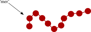 Figure 3: Schematic representation of a polymer
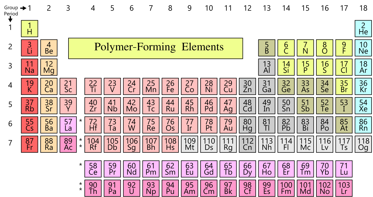
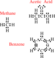 Figure 9: Examples of Lewis Diagrams
 Figure 10: Examples of Shorthand Notation when drawing chemical structures
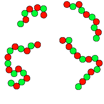 Figure 11: Polymers produced by step growth polymerization. The red and green circles correspond to 'A' and 'B' monomers that react with one another to form the polymer.
 Figure 12: Formation of an amide from an amine and a carboxylic acid
 Figure 13: Formation of an amide from a primary amine and an acid chloride
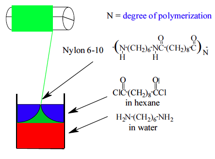 Figure 14: Schematic representation of the interfacial polymerization off nylon.
 Figure 15: Formation of an ester from an alcohol and a carboxylic acid.
 Figure 16: Ester hydrolysis: The reverse of the esterification reaction.
 Figure 17: Urethane Formation
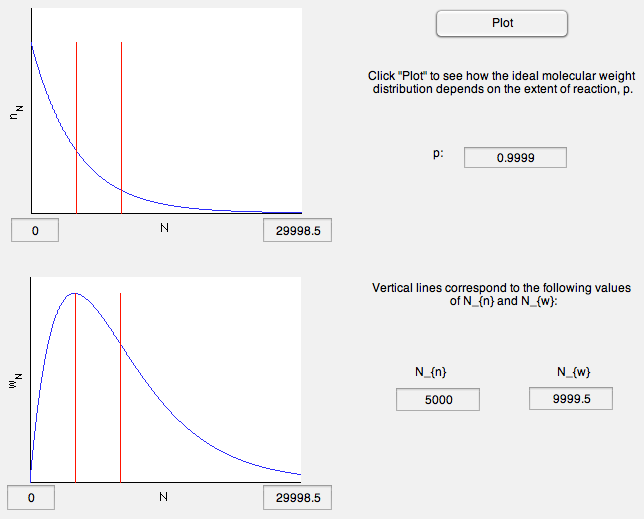 Figure 22: Distribution of molecular sizes during an ideal step growth polymerization.
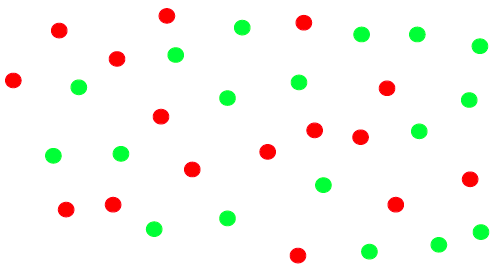 Figure 23: Nonlinear Step Growth Polymerization
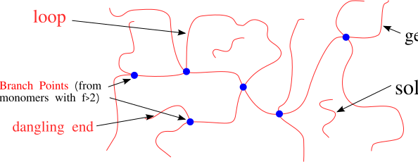 Figure 24: Molecular schematic of gel network.
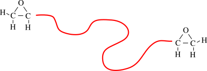 Figure 25: Example of a Prepolymer
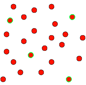
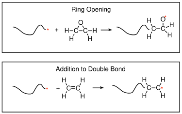


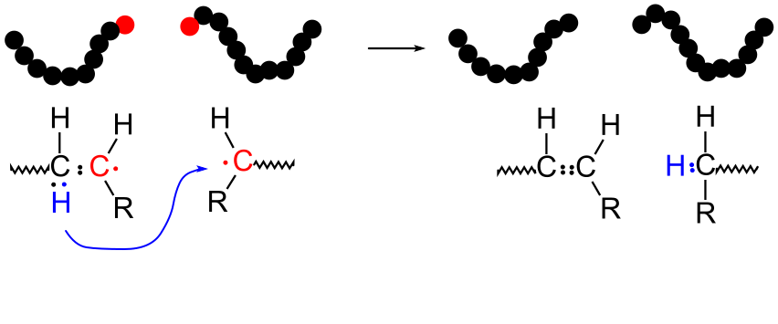
 Figure 34: Chain transfer to toluene.
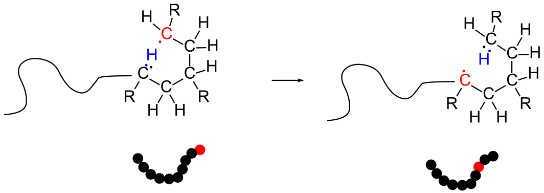
 Figure 38: Chemical structure of a vinyl monomer.
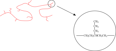


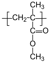

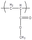

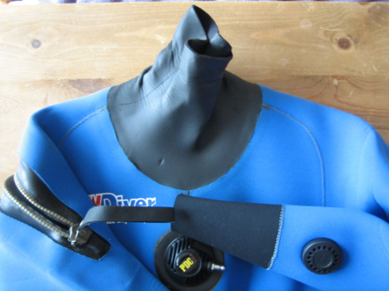


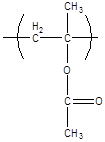
 Figure 54: Structure of poly(vinyl chloride)
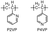


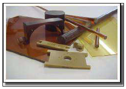


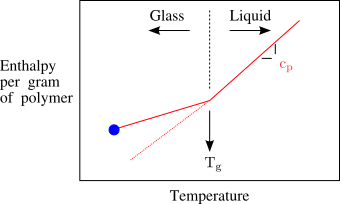


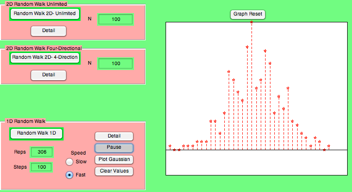
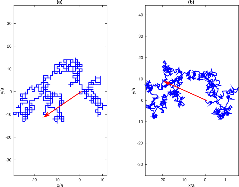
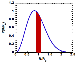
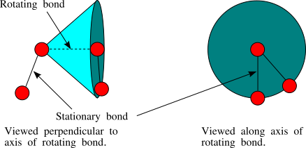
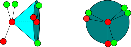
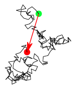
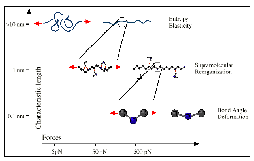
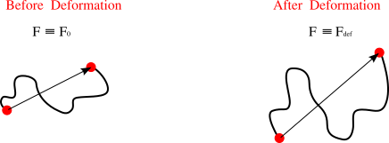



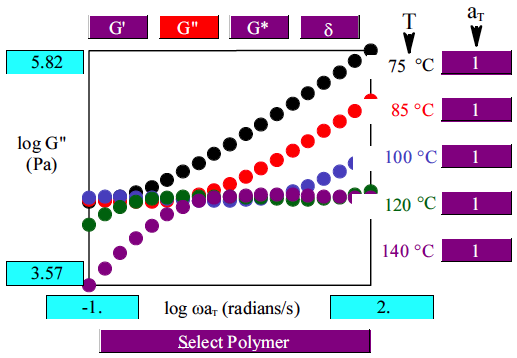
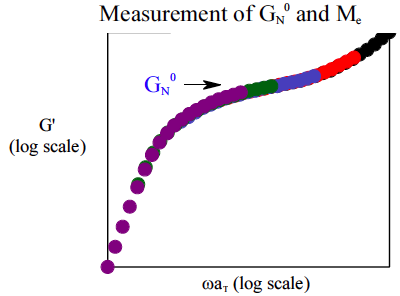
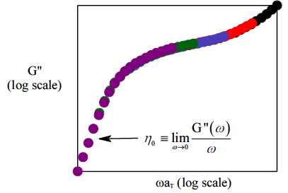
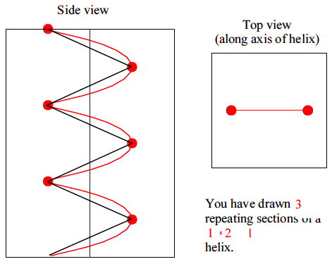
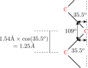
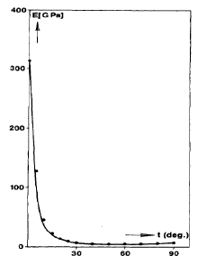


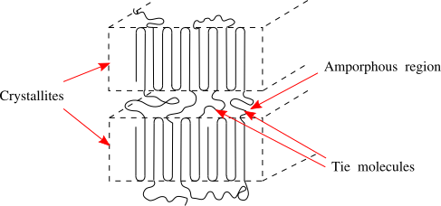

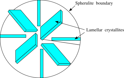
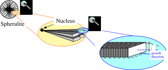

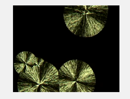
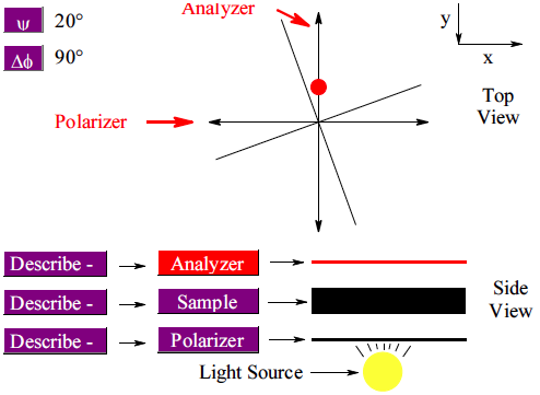
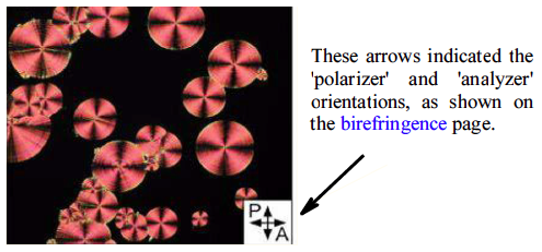
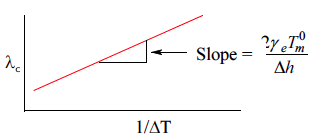
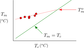
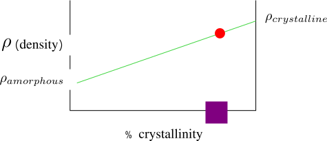

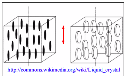
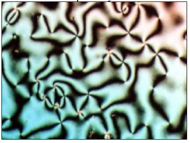
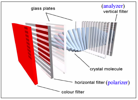
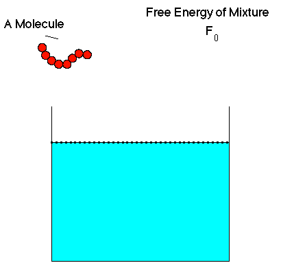
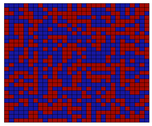


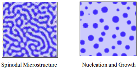
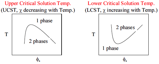
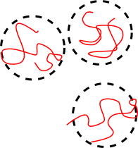
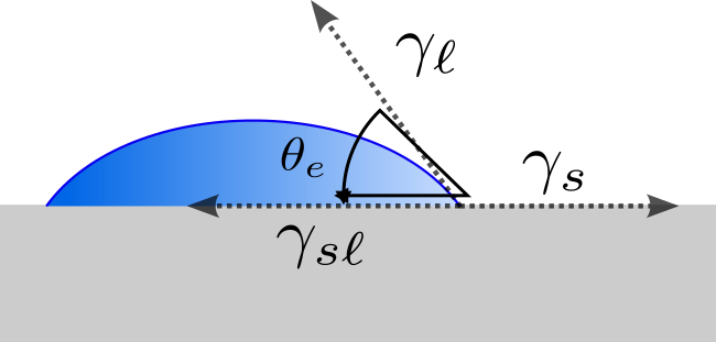
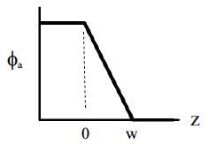
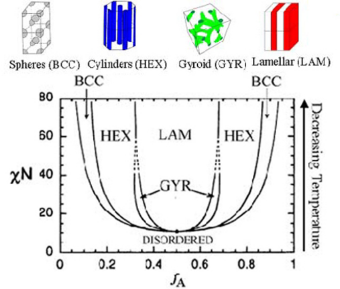 Figure 163: Block copolymer phase diagram (adapted from ref.[6]).
